Chalk talk: How to model air temperature variation with height
In his latest chalk talk, Dr. Colin Campbell, environmental scientist at METER Group, teaches how to model vertical variation in temperature and how to estimate sensible heat flux.
Video transcript
Hello, everyone. My name is Dr. Colin Campbell, and I’m a senior research scientist here at METER Group. For today’s chalk talk, we’ll be talking about modeling vertical variation in temperature. In Figure 1, I’ve put together a graph that shows the maximum and minimum temperature with height and depth in the soil at some snapshot in time at a particular place.

It’s interesting to note that the change in temperature with depth in the soil is much faster than the change in temperature with height, whether we’re talking about a maximum or minimum. And the reason is that even though air is a good insulator, it also mixes really well. And that mixing is caused by eddies. And there’s a little more to that story. It depends specifically on surface heating by the sun through radiation and the cover type, whether it’s plants, rocks, boulders, straight soil, snow, or wind.

If we were going to model that, we would start by writing an equation (Equation 1) where a temperature at sun height, Z, above the surface (see variables noted in Figure 1), is equal to an aerodynamic surface temperature, T0, minus the sensible heat flux, divided by 0.4 times rho, CP, which is the volume specific heat of the air, times a variable called u*, which is the friction velocity. We multiply all that by the logarithm of z, the height above the surface minus d, which is the zero plane displacement, divided by z h, which is a roughness parameter. You might notice up here in the list of variables, that the zero plane displacement is 0.6 times H. H is the canopy height in meters. The rough roughness parameter can be estimated as 0.02 times the canopy height or times H. Now we have an equation that will help us model temperature with height.
However, often we don’t know things like H, our sensible heat flux, and u*, our friction velocity. One of the things that we notice about this equation is that it’s set up somewhat like a linear equation. As you know, an example of a linear equation is something like Equation 2.

Figure 1 isn’t written quite that way, but if we look closely at the example below (Equation 3), this value could be our b, and this value our m, and this value could be our x. And if we do that, we actually can get some use out of graphing temperature with height.

So we went out one day and measured this with a METER Group set of environmental sensors set up at certain heights above the surface. Here we placed sensors at 0.2 m, 0.4 m, 0.8 m, and 1.6 m above the ground.

To visualize this, in Figure 2 we graphed height on the y axis and temperature on the x axis, similar to the graph in Figure 1.

We know from Equation 1 that the axes for temperature and height should be switched because temperature is the dependent variable, and height is the independent variable. So if we switch axes it would look like the graph in Figure 3.

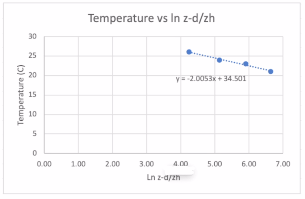
Figure 3 is graphed with the independent variable on the x axis and height on the y axis. If we fit this curve with today’s calculators, it would be fairly easy to get a curve that would fit that. But since it’s a linear equation, we can take the temperature data from Table 1 and the In ((Z-d)/ZH) data from Table 1 and graph them together.

Figure 4 is a graph that shows what happens when we do that. Notice that, just like we suggested, it creates a linear equation (Equation 4).

We learned in Figure 1 the B value was equal to t0 (our aerodynamic surface temperature). Since we know our surface temperature is 34.5 degrees, we can estimate what the temperature is down here at the surface, even though we only measured down 0.2 m.
We also know from Equation 4 that our M value is equal to -2.01. And if we look at Equation 1, our slope value is below.

So we can write

How to estimate sensible heat flux
Now, if we were interested in the sensible heat flux, which we often are, we can simply rearrange this equation to be

And in Figure 1, I forgot to give you this value, but for an air temperature of 20 degrees celsius,

And then finally, a typical unit for friction velocity, which should be measured in the field over the specific canopy you are in, is about 0.2 meters per second.

So if we did this calculation, we would learned that there’s about 193 watts per meter squared of sensible heat flux coming off that surface.

So if we can measure temperature at a few heights, we can estimate what the heat flux is coming off the surface assuming we know something about our canopy. Learn more about measuring and modeling environmental parameters at metergroup.com/environment. If you have any questions feel free to email Dr. Campbell at [email protected].
Learn more
Read about weather station best practices—>


