Skip to content

Posts from the ‘SRS NDVI sensor’ Category

Are floods and droughts really unpredictable?

In our latest podcast episode, Kevin Hyde, manager of the Montana Mesonet, discusses his views on predicting and mitigating the effects of flood and drought.

Montana’s large geographical area makes mesonet equipment maintenance a challenge.

He also shares how to build a robust weather network with high-quality data on a small budget, why setups should include other measurements such as soil moisture and NDVI, and the genius way he handles maintenance over such a large geographical area.

Listen now—>

Notes

Kevin Hyde is the manager of the Montana Mesonet. Learn more about the Montana Mesonet project on their website. 

Montana Mesonet website

Subscribe:

https://www.metergroup.com/we-measure-the-world/

Follow us:

Questions?

Our scientists have decades of experience helping researchers and growers measure the soil-plant-atmosphere continuum. 

Disclaimer

The views and opinions expressed in the podcast and on this posting are those of the individual speakers or authors and do not necessarily reflect or represent the views and opinions held by METER.

Episode 9: Pioneers of Environmental Measurement

What was the life of a scientist like before modern measurement techniques? In our latest podcast, Campbell Scientific’s Ed Swiatek and METER’s Dr. Gaylon Campbell discuss their association with three pioneers of environmental measurement.

Learn what it was like to practice science on the cutting edge. Discover the creative lengths they went to and what crazy things they cobbled together to get the measurements they needed.

Listen now—>

Smart orchard aims to install thousands of sensors for actionable insights

When big data is a problem

Orchard growers today live in an exciting time where environmental data are becoming inexpensive and abundant. But going from a data-poor to a data-rich environment has its challenges. Big data can be so overwhelming that growers struggle with how to turn that data into actionable insight.

In March, Innov8.ag began piloting a smart orchard project in collaboration with researchers from Washington State University & Oregon State University at Chiawana Orchards in Washington state.

One grower on the Washington Tree Fruit Research Commission recently commented that he uses no less than 19 data apps for making decisions. Steve Mantle, founder of innov8.ag, says, “It’s just overwhelming to a grower to consolidate all of this data together. We need to figure out how to help them with actual insights that impact either their yield quality / quantity—and just as importantly—their costs: particularly on labor, chemical/nutrients, and irrigation.”  That’s why in 2020, Mantle and his team approached the Tree Fruit Research Commission’s technology committee to see if they could bring their capabilities, ingesting data from many different data silos and sensor providers into one place, with the goal of providing actionable insights for growers in the apple orchard space. Thus, the idea of a “smart orchard” was born.

Turning big data into a solution

In March, Innov8.ag began piloting a smart orchard project in collaboration with researchers from Washington State University & Oregon State University at Chiawana Orchards in Washington state. Their goal was to “sensorize” an orchard from multiple hardware providers, bringing together growers, data, and researchers to create a sustainable, “smart” orchard with insights that impacted a grower’s bottom line. To do this they combined data from on-farm and off-farm, online and offline sources including satellites, drones, weather providers, telemetry from IoT devices such as soil moisture probes and leaf wetness sensors, and more.” Mantle adds, “We’re trying to see how the sensors at different price points and from different vendors compare against each other in terms of accuracy. But the biggest goal is to get more granularity around and prove the value in canopy, soil, and weather measurements. Then we tie that in with yield, quality, and profit.”

Installing sensors so that comparisons are valid

The smart orchard consists of 100 rows of Gala apple trees spaced out over two 20-acre blocks. A number of different sensor/instrumentation providers, including METER Group, have their sensors deployed at this smart orchard measuring parameters such as weather, irrigation, soil water and nutrients, chemicals, disease, pests, crop health, labor, and drone/satellite imagery. All these data are aggregated and organized on a regular basis to try and enable growers to better understand weather and climate change to make precise, informed decisions and better manage their water usage, labor, equipment, and chemical usage.

Smart Orchard team member and researcher, Harmony Liu, says one challenge they face is making sure the comparisons are valid. “We are careful to install the same sensor types at the same heights so we are making “apple-to-apple” comparisons.”

Liu says in addition to sensing, they collect soil samples every week throughout the season and send them out to two different labs for nutrient testing so they can look at how that data compares with the soil nutrient sensors. They sample at five different locations at three different depths to match the sensors. She adds, “We have the dendrometer, soil nutrient data, soil moisture data, and canopy data all being collected within the same zone. It’s part of our intent to show this data all connecting with each other.” The team also measures irrigation line pressure with a sensor as opposed to using an irrigation switch. Liu says, “We want to know what the pressure signature is as everything turns on and activates so we can understand what that signature looks like and start to identify when there are abnormalities in how the irrigation system fills.” Additionally, they’re using METER NDVI and PRI sensors as well as a pyranometer for ground truthing the drone imagery that they’re doing at a 7 centimeters per pixel resolution.

The goal is understanding in-canopy weather and how to work with institutions on adapting models for disease, pests, and ultimately informing spray management.

Data cleanup is time-consuming

Liu says getting the smart orchard up and running was not without its challenges. “The first challenge was gaining access to some of the data from grower owned instruments because those instruments are not all grouped together.” Liu says that challenge made data cleanup time consuming, but they worked their way through it. She adds, “Overall, having this density of data is difficult because it’s a lot to wade through. But at the same time, it’s been really helpful. Data has been reliable coming in across the board.”

In-farm vs. outside-farm measurements

Liu says one thing they are interested in is accurately measuring temperature and humidity within the orchard because these parameters are critical for apple disease modeling. She says, “When people are modeling disease, they take the inputs from weather forecasts into the disease model for risk calculations. But there are some differences in environmental conditions inside vs. outside the orchard where evapotranspiration will cause temperatures in the canopy to be cooler compared to outside-farm temperatures while the vapor pressure is higher. So that’s one thing we use METER group instruments for. We have outside-orchard,  above-orchard, and in-canopy ATMOS 41 weather stations and ATMOS 14 temperature and relative humidity sensors. We use these to compare the temperature and relative humidity difference. By using an instrument from the same provider, we eliminate the systematic bias vs. if we were to compare temp and RH from different providers. We also set up a vertical profile by installing sensors on the same pole at different heights and could see how the temperature and humidity changed across height for that location.”

Register for the smart orchard project live webinar with innov8.ag this Thursday, Jan.14th at 4pm PST.

Future smart orchard goals

Mantle says their most important goal is understanding in-canopy weather and how they can work with WSU and other institutions on adapting models for disease, pests, and ultimately informing spray management. Liu adds, “We also want to understand data comparison and unification. We want to bring together soil moisture measurements like volumetric water content and data from the METER TEROS 21 matric potential sensor. What we found is that, although they’re looking at soil moisture from different perspectives, unifying the two measurements will be critical for people working on irrigation scheduling.” The team also plans on working with WSU professors to create an evapotranspiration map that blends together some of the sensor telemetry and the view from a drone.

See the webinar

Want to learn more? METER soil physicist, Dr. Colin Campbell and Washington State University soil scientist Dr. Dave Brown discuss the smart orchard project in a METER Group webinar.

View more METER crops webinars—>

Learn more

Download the “Complete guide to irrigation management”—>

Why mesonets make weather prediction more accurate

The staggering cost of Montana’s “flash drought”

Some people figured it was climate change. One statistician said it was a part of a cyclical trend for poor crop years. Whatever the cause, the 2017 flash drought that parched the entire state of Montana and most of South Dakota, severely impacted the profitability of ranchers and farmers. In western Montana, fires burned some of the largest acreages in recent history. It resulted in one of the biggest wildfire incident reports (over one-million acres) and caused virtually 100% crop loss in northeastern Montana. The U.S. Dept. of Agriculture estimated the crop loss to be in the hundreds of millions of dollars, and one question was on everybody’s mind—why did no one see it coming?

Montana drought status chart

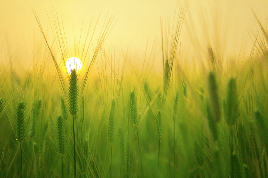
Figure 1. Montana drought conditions August 2017 (Source: Montana State Library website: https://mslservices.mt.gov/Geographic_Information/Maps/drought/)

Getting the right weather data

The 2017 Montana Dept. of Natural Resources and Conservation spring drought report indicated plenty of water: “By the end of the month, almost all drought concern was removed from the state, with the exception of Wibaux and Fallon Counties….As of May 9, 2017, Montana was 98.45% drought free.” But in late May, an abrupt shift in weather conditions led to one of the hottest, driest summers on record.

The problem, says Kevin Hyde, Montana State Mesonet Coordinator, lies not only in the need for more weather data but in obtaining the right kind of data. He says, “One of the reasons drought was missed was because we’re still thinking you measure drought by snowpack and how much water is in the river, which is really great if you’ve got water rights. But we’ve got a lot of dryland out there.”

In addition to weather monitoring, Hyde is a big proponent of adding soil moisture and NDVI measurements to each of the Montana Mesonet stations he oversees. He says, “The conventional weather station only measures atmospheric conditions. But ultimately, to make any decisions, we’ve got to know not just how much water comes into the system, but how much goes into the soil. And even that’s not enough…because what we really need to know is how the water situation is going to affect plants.”

Hyde says more data are needed to warn growers and ranchers about upcoming weather risks. He points to the fact that increasing evapotranspiration got missed leading up to the summer of 2017. “We realized that if we were looking carefully at reference ET, we might have seen it about a month earlier. What would people have done? They would have changed their calf purchases. They would have figured out what kind of forage they needed to buy. These are the types of decisions people can make if they know the information sooner.”

Was the drought over? Soil moisture illuminates the bigger picture

Heavy rains came mid-September of 2017, which led some people to believe the drought was over. However, changes in soil moisture told a different story. Very little of the rain made it into the soil. “At the Havre, MT station you can see we had some heavy precipitation events. Then we had early October snows. So people expected good soil water recharge. But at the end of the day, we didn’t get it. On Sept.15th, soil moisture sensors showed a big soil moisture response at the surface but only a marginal response at 8 inches.” The melt of early October snows onto the soil, still damp from the September rain, drained to 20 inches or more. But as the snowmelt dissipated, there was minimal net gain going into the winter.

Soil moisture chart for Montana

Figure 2. Soil moisture traces at the Havre, MT weather station

Predictive models need more coverage to be effective

Typically in the U.S., the National Weather Service (a division of NOAA) puts out a network of weather monitoring stations spaced out across the country, and that data gets fed into forward-looking models that help predict the weather. Dr. Doug Cobos, research scientist at METER says, “What people are finding out is that putting in a sparse network of very expensive systems has done really well. It’s been a good thing. But the spatial gaps in those networks are a problem, especially for agriculture producers and ranchers. They need to know what’s happening where they are.”

Hyde agrees, adding that we need better predictive tools that help growers and ranchers make practical decisions based on data rather than guessing. “January 1st is when the decision has to be made—do I buy cows? Do I sell cows? Do I need more pasture? But many predictions start on April 1st. As one rancher puts it, ‘We don’t bother with Las Vegas. We sit around the dining room table at the beginning of the year and put a million dollars on one shot.’”

Mesonets improve spatial distribution

Mesonets present a practical solution for the need to fill in data gaps between large, complex weather stations. The Montana Mesonet currently has 57 stations interspersed throughout the state, and through partnerships with both the public and private sector, they’re adding more stations every year.

Map of mesonet weather stations

Figure 3. Map of MT Mesonet weather stations (source: http://climate.umt.edu/mesonet/)

At each location, the Montana Mesonet team installs METER all-in-one weather stations, soil moisture sensors, NDVI sensors and data loggers that integrate with ZENTRA Cloud: an easy-to-use web software that seamlessly integrates into third-party applications through an API. He says the system enables better spatial distribution and reliability. “When we were deciding on equipment we asked ourselves: What kind of technology should we use? It had to provide high data integrity. It had to be easy to deploy and maintain. And it had to be cost effective. There’s not a lot of people in that sector. METER systems are low profile, they’re affordable, and the reliability is there. I look at some other mesonets, and they cannot afford to build out further because they are relying on large, complex, expensive systems. That’s where the METER system comes into play.”

Montana mesonet weather station setup

Figure 4. Montana Mesonet station setup (Photo credit: Kevin Hyde)

Betting on the future

The Mesonet team and its partners are excited to see how their data will mesh with the available predictive tools to be the most useful and practical for growers and ranchers throughout the state, and they realize that there is still much work to do. “It’s not enough just to get the instrumentation out there. The overall crux is: how do we build the information network, and how do we build a relationship with the producers so that we can have an iterative and interactive conversation?” says Hyde. “We know there needs to be an education in how to use and interpret the data. For example: what is NDVI, and what can we learn from it? A lot of what we need to do is translate science into practical terms.” But he adds that it doesn’t need to be perfect. “What the farmers have said to us is, ‘We don’t need exact numbers. We’re gamblers. Give us probability. Teach us what it means, and we’ll make the decision.’”

Find more information on the Montana Mesonet here and in their newsletter.

See weather sensor performance data for the ATMOS 41 weather station.

Explore which weather station is right for you.

Download the “Researcher’s complete guide to soil moisture”—>

IoT Technologies for Irrigation Water Management (Part 2)

Dr. Yossi Osroosh, Precision Ag Engineer in the Department of Biological Systems Engineering at Washington State University, continues (see part 1) to discuss the strengths and limitations of  IoT technologies for irrigation water management.

Grapes being irrigated

Informed irrigation decisions require real-time data from networks of soil and weather sensors at desired resolution and at a reasonable cost.

LoRaWAN (a vendor-managed solution see part 1) is ideal for monitoring applications where sensors need to send data only a couple of times per day with very high battery life at a very low cost. Cellular IoT, on the other hand, works best for agricultural applications where sensors are required to send data more frequently and irrigation valves need to be turned on/off. Low-Power Wide-Area Networking (LPWAN) technologies need gateways or base stations for functioning. The gateway uploads data to a cloud server through traditional cellular networks like 4G. Symphony Link has an architecture very similar to LoRaWAN with higher degree of reliability appropriate for industrial applications. The power budget of LTE Cat-M1 9 (a network operator LPWAN) is 30% higher per bit than technologies like SigFox or LoRaWAN, which means more expensive batteries are required. Some IoT technologies like LoRa and SigFox only support uplink suited for monitoring while cellular IoT allows for both monitoring and control. LTE-M is a better option for agricultural weather and soil moisture sensor applications where more data usage is expected.

NB-IoT is more popular in EU and China and LTE Cat-M1 in the U.S. and Japan. T-Mobile is planning to deploy NB-IoT network in the U.S. by mid-2018 following a pilot project in Las Vegas. Verizon and AT&T launched LTE Cat-M1 networks last year and their IoT-specific data plans are available for purchase. Verizon and AT&T IoT networks cover a much greater area than LoRa or Sigfox. An IoT device can be connected to AT&T’s network for close to $1.00 per month, and to Verizon’s for as low as $2 per month for 1MB of data. A typical sensor message generally falls into 10-200 bytes range. With the overhead associated with protocols to send the data to the cloud, this may reach to 1KB. This can be used as a general guide to determine how much data to buy from a network operator.

Fruit on a tree branch

Studies show there is a potential for over 50% water savings using sensor-based irrigation scheduling methods.

What the future holds

Many startup companies are currently focused on the software aspect of IoT, and their products lack sensor technology. The main problem they have is that developing good sensors is hard. Most of these companies will fail before the batteries of their sensors die. Few will survive or prevail in the very competitive IoT market. Larger companies that own sensor technologies are more concerned with the compatibility and interoperability of these IoT technologies and will be hesitant to adopt them until they have a clear picture. It is going to take time to see both IoT and accurate soil/plant sensors in one package in the market.  

With the rapid growth of IoT in other areas, there will be an opportunity to evaluate different IoT technologies before adopting them in agriculture. As a company, you may be forced to choose specific IoT technology. Growers and consultants should not worry about what solution is employed to transfer data from their field to the cloud and to their computers or smartphones, as long as quality data is collected and costs and services are reasonable. Currently, some companies are using traditional cellular networks. It is highly likely that they will finally switch to cellular IoT like LTE Cat-M1. This, however, may potentially increase the costs in some designs due to the higher cost of cellular IoT data plans.

IoT Technologies Chart

Download the “Researcher’s complete guide to water potential”—>

Download the “Researcher’s complete guide to soil moisture”—>

Download the “Researcher’s complete guide to SDI-12″—>

Get more info on applied environmental research in our

Learn more

Download the “Complete guide to irrigation management”—>

How to Get More From Your NDVI Sensor (Part 3)

In the conclusion of our three-part series on improving NDVI sensor data (see part 2), we discuss how to correct for limitations which occur in high leaf area index (LAI) conditions.

NDVI Sensor

Where there’s a large amount of vegetation, NDVI tends to saturate.

NDVI Limitations – High LAI

NDVI is useful in the midrange of LAI’s as long as you don’t have strong soil effects, but as you approach an LAI above 4, you lose sensitivity. In figure 6, loss of sensitivity is primarily due to a saturation in the red band. Measurements were taken in a wheat canopy and a maize canopy. The near-infrared reflectance is sensitive across the entire spectrum of the wheat and maize canopies, but the red saturates relatively quickly. Where the red starts to saturate is where the NDVI starts to saturate.

NDVI Sensor

Figure 6: Gitelson (2004) J. Plant Phys

Note: NDVI saturates at high LAI’s, however, if your purpose is to get at the fractional interception of light, NDVI tends not to have the saturation issue. In Figure 7, Fpar or the fractional interception of light of photosynthetically radiation is nearly complete far before NDVI saturates. This is because canopies are efficient at intercepting light, and once we get to an LAI of about 4, most of the light has been intercepted or absorbed by the canopy.  Thus, incremental increases in LAI don’t significantly affect the FPar variable.

NDVI Sensor

Figure 7: Fractional interception of light is near complete at an LAI around 4. (Gamon et al. (1995) Eco. Apps)

Solution 3- WDRVI

One solution for the NDVI saturation issue is called the Wide Dynamic Range Vegetation Index (WDRVI). Its formulation is similar to NDVI, except for a weighting coefficient that can be used to reduce the disparity between the contribution of the near infrared and red reflectance.  

NDVI Sensor

In the WDRVI, a is multiplied by the near-infrared reflectance to reduce its value and bring it closer to the red reflectance value. In doing so, it balances out the red and the near-infrared contribution to the vegetation index.

NDVI Sensor

Figure 8: (Gitelson (2004) J. Plant Phys)

a can range anywhere from 0 to 1. Figure 8 shows that as we use a smaller value of a, we get an increasing linear response of the wide dynamic vegetation index to LAI.

The only drawback of the WDRVI is that the selection of a is subjective. It’s something that you experiment on your own until you find a value for a that is optimal for your solution.  People tend to err on the side of a very low value simply because they’ll get closer and closer to a linear response to LAI as a decreases.

Solution 4 – Enhanced Vegetation Index

The enhanced vegetation index (EVI) was designed to enhance sensitivity in high biomass ecosystems, but it also attempts to reduce atmospheric influences.  This was a vegetation index created for the purposes of a satellite-based platform. There’s a lot of atmosphere to look through from a satellite to the ground, and sometimes the aerosols in the atmosphere affect the reflectances in the red and the near infrared regions causing spurious observations.  The EVI also tries to reduce sensitivity of the index to soil. Thus the EVI is a kind of solution to both extremes.

NDVI Sensor

In the EVI equation, the two major inputs are near infrared and red reflectances.  C1 , C2, and L are all parameters that can be estimated, but the blue band is something that has to be measured. Most NDVI sensors are two band sensors, so you don’t have that information in the blue.  Plus, with satellites, the blue band is relatively noisy and doesn’t always have the best quality data, thus EVI has limited value.

Solution 6: EVI2 (Enhanced Vegetation Index 2)

Those problems led a scientist named Jiang to come up with a solution.  Jiang observed quite a bit of autocorrelation between the red band and the blue band, so he decided to try and formulate EVI without the blue band in what he called the EVI2 (Enhanced Vegetation Index 2).  if you’re interested in the mathematics, we encourage you to read his paper, but here we give you the equation in case you’re interested in using it.

NDVI Sensor

Figure 9

When Jiang calculated his EVI2 and compared it to the traditional EVI (Figure 9), it was nearly a one to one relationship. For all intents and purposes EVI2 was equivalent to EVI.  Since this avoids blue band, it offers some exciting possibilities as it reduces to just using the two inputs of NIR and red bands to calculate NDVI.

NDVI Sensor Summary

NDVI measurements have considerable value, and though there are extremes where NDVI performs poorly, even in these cases there are several solutions.  These solutions all use the near infrared and the red bands, so you can take an NDVI sensor, obtain the raw values of NIR and red reflectances and reformulate them in one of these indices (there are several other indices available that we haven’t covered). So if you’re in a system with extremely high or low LAI, try to determine how near infrared and red bands can be used in some type of vegetation index to allow you to research your specific application.

Download the “Researcher’s complete guide to soil moisture”—>

Download the “Researcher’s complete guide to leaf area index (LAI)”—>

Get more information on applied environmental research in our

Get More From Your NDVI Sensor (Part 2)

Last week we discussed Normalized Difference Vegetation Index (NDVI) sampling across a range of scales both in space and in time, from satellites sampling the entire earth’s surface to handheld small sensors that measure individual plants or even leaves (see part 1).  This week, learn about NDVI applications, limitations, and how to correct for those limitations.

Field with crop seedlings starting to sprout

Limitations of the Normalized Difference Vegetation Index tend to occur at the extremes of the spectrum.

Green crops in a field

NDVI Applications

People use NDVI to infer things like leaf area index (LAI) or fractional light interception (FPAR) of a canopy.  Some scientists also associate NDVI with biomass or yield of a crop. People also use NDVI to get a sense of phenology (general temporal patterns of greenness), as well as where vegetation occurs or how much vegetation is in a particular location.

In Figure 4, you can see how the reflectance spectrum at a given canopy LAI changes with leaf area index, decreasing in the visible range while increasing in the near infrared.

Diagram depicting NDVI Sensor data

Figure 4

At very low LAI’s, the reflectance spectrum is relatively undifferentiated between red and NIR (black line), but when LAI is high, there’s a strong absorption of red light by chlorophyll with a strong reflectance in the NIR. In fact, as LAI increases, there’s an ever-increasing reflectance in the near infrared around 800 nm.

NDVI Limitations

Limitations of the Normalized Difference Vegetation Index tend to occur at the extremes of the spectrum. Any time there’s very low vegetation cover (majority of the scene is soil), NDVI will be sensitive to that soil. This can confound measurements.  On the other extreme, where there’s a large amount of vegetation, NDVI tends to saturate. Notice the negligible difference between spectra at a leaf area index (LAI) of 3 (purple) versus 6 (green). Indeed, in a tropical forest, NDVI will not be sensitive to small changes in the LAI because LAI is already very high.  However, several solutions exist.

Solution 1-Soil Adjusted Vegetation Index

Figure 5 shows the results of a study taking spectral measurements of different vegetation indices across a transect of bare soil.  Moving from dry clay loam to wet clay loam, we see a very strong response of NDVI due to the wetness of the soil; undesirable if we’re measuring vegetation.  We’re not interested in an index that’s sensitive to changes in soil or soil moisture. However, there are a few other indices plotted in figure 5 with much lower sensitivities to variations in the soil across the transect.

Diagram of Maricopa Aircraft Data

Figure 5: Qi et al. (1994) Rem. Sens. Env.

The first one of those indices is the Soil Adjusted Vegetation Index (SAVI). The equation for SAVI is similar to NDVI. It incorporates the same two bands as the NDVI—the near infrared and the red.

Image depicts two equations one is NDVI and the other is SAVI

Soil Adjusted Vegetation Index (Huete (1988) Rem. Sens. Env.)

The only thing that’s different, is the L parameter.  L is a soil adjustment factor with values that range anywhere from 0 to 1.  When vegetation cover is 100%, L is 0 because there’s no need for a soil background adjustment. However, when vegetation cover is very low, that L parameter will approach one. Because it is difficult to measure exactly how much vegetation cover you have without using NDVI, we can modify the NDVI so it’s not sensitive to soil by guessing beforehand what L should be. It’s common practice to set L to an intermediate value of 0.5. You can see in Figure 5 the Soil Adjusted Vegetation Index or SAVI has a much lower sensitivity to the soil background.

Solution 2- Modified SAVI

The next vegetation index is the modified SAVI (MSAVI). The SAVI equation contains an L parameter that we have to estimate—not an accurate way of handling things.  So a scientist named Key developed a universal optimum for L. We won’t get into the math, but he was able to simplify the SAVI equation to where there’s no longer a need for the L parameter, and the only inputs required are the reflectances in the near infrared and the red.  

Image depicts two equations SAVI is the top equation while the bottom equation is modified SAVI or MSAVI

Modified SAVI (Qi et al. (1994) Rem. Sens. Env.)

This was a pretty significant advance as it circumvented the need to estimate or independently measure L. When Key compared SAVI to MSAVI, there was virtually no difference between the two indices in terms of their sensitivity to the amount of vegetation and their response to the soil background.

Depicts a compairson of MSAVI and SAVI in terms of dynamic range and noise level

MSAVI compares well with SAVI in terms of dynamic range and noise level (Qi et al. (1994) Rem. Sens. Env.)

Next week:  Learn about solutions for high LAI.

Download the “Researcher’s complete guide to soil moisture”—>

Download the “Researcher’s complete guide to leaf area index (LAI)”—>

Get more information on applied environmental research in our

Get More From Your NDVI Sensor

Modern technology has made it possible to sample Normalized Difference Vegetation Index (NDVI) across a range of scales both in space and in time, from satellites sampling the entire earth’s surface to handheld small sensors that measure individual plants or even leaves.

Flat map of the earth depicting NDVI amounts covering the contents

Figure 1: NDVI is sensitive to the amount of vegetation cover that is present across the earth’s surface.

NDVI – Global

The broadest way to think of NDVI is data obtained from an earth orbiting satellite. In the figure above, you can see highly vegetated areas that have high NDVI values represented by dark green colors across the globe.  Conversely, areas of low vegetation have low NDVI values, which look brown.  NDVI is sensitive to the amount of vegetation cover that is present across the earth’s surface.

NDVI – Local

How might NDVI be useful at the plot level? Figure 2 below shows a successional gradient where time zero is a bare patch of soil, or a few forbs or annual grasses. If we leave that patch of ground for enough time, the vegetation will change: shrubs may take over from grasses and eventually we might see a forest. Across a large area, we may also move from grasslands to forest. In an agricultural system, there is yearly turnover of vegetation—from bare field to plant emergence, maturity, and senescence. This cycle repeats itself every year.  Within these growth cycles NDVI helps to quantify the canopy growth that occurs over time as well as the spatial dynamics that occur across landscapes.

Diagram depicting seasonal growth plotted against spatiotemporal variation

Figure 2: Seasonal growth plotted against spatiotemporal variation

Spectral Reflectance Data

So where does NDVI come from? In Figure 3, the x-axis plots wavelength of light within the electromagnetic spectrum; 450 to 950 nm covers both the visible region and a portion of the near infrared. On the y-axis is percent reflectance.  This is a typical reflectance spectrum from green vegetation.

Chart reflecting data and electromagnetic radiation

Figure 3: Spectral Reflectance Data. (Figure and Images: landsat.gsfc.nasa.gov)

The green hyperspectral line is what we would expect to get from a spectral radiometer.  Reflectance is typically low in the blue region, higher in the green region, and lower in the red region. It shifts dramatically as we cross from the visible to the near infrared. The two vertical bars labeled NDVI give you an idea of where a typical NDVI sensor measures within the spectrum.  One band is in the red region and the other is in the near-infrared region.  

NDVI capitalizes on the large difference between the visible region and the near infrared portion of the spectrum. Healthy, growing plants reflect near-infrared strongly.  The two images on the right of the figure above are of the same area.  The top image is displayed in true color, or three bands–blue, green and red. The image below is a false color infrared image.  The three bands displayed are blue, green, and in place of red, we used the near infrared. The bright red color indicates a lot of near infrared reflectance which is typical of green or healthy vegetation.

The reason NDVI is formulated with red and near infrared is because red keys in on chlorophyll absorption, and near infrared is sensitive to canopy structure and the internal cellular structure of leaves.  As we add leaves to a canopy, there’s more chlorophyll and structural complexities, thus we can expect decreasing amounts of red reflectance and higher amounts of near-infrared reflectance.

How Do We Calculate the NDVI?

Calculation equation of NDVI

The Normalized Difference Vegetation Index takes into account the amount of near-infrared (NIR) reflected by plants. It is calculated by dividing the difference between the reflectances (Rho) in the near-infrared and red by the sum of the two.  NDVI values typically range between negative one (surface water) and one (full, vibrant canopy). Low values (0.1 – 0.4) indicate sparse canopies, while higher values (0.7 – 0.9) suggest full, active canopies.  

The way we calculate the percent reflectance is to quantify both the upwelling radiation (the radiation that’s striking the canopy and then reflected back toward our sensor) as well as the total amount of radiation that’s downwelling (from the sky) on a canopy.  The ratio of those two give us percent reflectance in each of the bands.

Next Week: Learn about NDVI applications, limitations, and how to correct for those limitations.

Download the “Researcher’s complete guide to soil moisture”—>

Get more information on applied environmental research in our

Measuring NDVI in a Greenhouse Presents Challenges (Part 2)

University of Georgia researcher, Shuyang Zhen, wanted to find out if she could optimize greenhouse irrigation with reference evapotranspiration calculated from environmental factors and a crop coefficient, using NDVI measurements to adjust for canopy size (see part 1). Learn the results of the experiment and how fast growth and flowering caused problems with the NDVI measurement.

Researchers measuring the NDVI of green plants in a greenhouse

Shuyang’s experimental setup.

Fast Growth Causes Problems

Shuyang says because the plants grew so large, the canopy filled in beyond what the sensor could see.  That meant there was additional leaf area that participated in vapor loss which wasn’t identified by the NDVI sensor.  As the canopies approached moderate-to-high canopy densities, Shuyang observed that the NDVI readings became less responsive to increases in canopy size. To work around this problem, Shuyang tried to calculate a vegetation index called the Wide Dynamic Range Vegetation index with the spectral reflectance outputs of the two wavebands measured by the NDVI sensor. Shuyang says, “This index was supposed to improve the sensitivity at higher canopy density, so I transformed all my data and was surprised that it actually improved the sensitivity when the canopy density was lower.  But at a higher canopy density it wasn’t as effective.”

Researchers measuring NDVI of petunias in a greenhouse

The red flowers reflected a lot of red light compared to the leaves, which confused the NDVI measurement.

Plant flowering also caused problems with the NDVI measurement.   Shuyang explains, “We had one cultivar of petunia with red flowers which formed on top of the canopy. The red flowers reflected a lot of red light compared to the leaves, which confused the NDVI measurement.  The NDVI value gradually decreased when the plants started to flower. There was no way I could get around that issue, so in some of the replicates, I removed the flowers, and in some I kept the flowers so I could compare the different responses and characterize why it happened.”

Poinsettia plant with red small flowers

The NDVI was very sensitive to the increase in crop size when the canopy was relatively small, but when you reach a certain canopy size and the canopy closure was nearly complete, then the sensitivity decreased.

Summary and Future Studies

During the early stages of growth, the research team saw a linear relationship between NDVI and crop coefficient. However, when the crop coefficient reached higher values, the response leveled off.  Shuyang says, “The response failed to change with further increases in the crop coefficient. The NDVI was very sensitive to the increase in crop size when the canopy was relatively small, but when you reach a certain canopy size and the canopy closure was nearly complete, then the sensitivity decreased.”  

Six poinsettia plants with small flowers arranged with one in the middle and five around the middle one in a circle

Lack of NDVI sensitivity during canopy closure and flowering translated to a problem with under-irrigation,

Shuyang adds that the lack of NDVI sensitivity during canopy closure and flowering translated to a problem with under-irrigation, so the team is thinking about developing separate models for different canopy stages.  She explains, “When the canopy reaches high canopy closure we may have to add an additional coefficient to compensate for that underestimation, but it’s difficult to evaluate what kind of coefficient we should use without more data. We need to do more studies to get an idea of what kind of adjustments will make the prediction more precise.”

Learn more about Shuyang’s work on the University of Georgia horticulture blog.

Download the “Researcher’s complete guide to soil moisture”—>

Get more information on applied environmental research in our

Measuring NDVI in a Greenhouse Presents Challenges

Greenhouse growers need irrigation strategies to maintain high plant quality, but it’s difficult to obtain quantitative information on exactly how much water will produce the highest-quality growth.

Picture of green house full of bright red Poinsettia plants

Greenhouse plant canopies are highly variable.

Estimating irrigation needs by using reference evapotranspiration calculated from environmental factors and a crop coefficient is standard for controlling field crop irrigation, but in a greenhouse this method can be challenging.  Greenhouse plant canopies are highly variable, and there’s limited information on the crop coefficient values for ornamental crops.  

Sensor-controlled, automated irrigation system in a greenhouse

Researchers used a sensor-controlled automated irrigation system with soil moisture sensors.

Measuring Crop Size

University of Georgia researcher, Shuyang Zhen, wanted to find out if she could solve this problem for greenhouse growers using NDVI measurements to adjust for canopy size. In a greenhouse setting, she and her team planted four types of fast growing herbaceous plants in small containers on top of greenhouse benches.  They set up a small weather station to monitor environmental parameters and used that data to calculate reference evapotranspiration.  

Green plants being monitored in a greenhouse

NDVI measurements are a non-destructive, continuous monitoring method to get information as to how big a crop is.

Using a sensor-controlled automated irrigation system with soil moisture sensors, the team determined the amount of water the plants used, which allowed them to calculate a crop coefficient on a daily basis.  They then used NDVI measurements to monitor crop size.  Shuyang says, “It’s easy to monitor environmental factors such as light, temperature, relative humidity, and wind speed, but it’s much harder to determine how big the crop is because many methods are destructive and time-consuming.  We chose NDVI measurements as a non-destructive, continuous monitoring method to get information as to how big our crop was. We were specifically interested in looking at how NDVI changes with the crop coefficient and how those two parameters correlate with each other.”

Purple flowers blooming in a greenhouse

Some species were more upward growing and some more sprawling.

Shuyang mounted multiple NDVI sensors on top of the benches, approximately four feet from the plants. Each sensor had a field of view of about .6 square meters and tracked the changes in plant size and NDVI values for over 8 weeks.  Shuyang says, “Each species had different growth habits.  Some species were more upward growing and some more sprawling. They also had different leaf chlorophyll content. Over the course of my study, three species reached reproductive stages, producing flowers. All of these factors had an effect on the NDVI measurements.”

Next week: Learn the results of the experiment and how fast growth and flowering caused problems with the measurement.

Download the “Researcher’s complete guide to soil moisture”—>

Get more information on applied environmental research in our