You’ve buried soil water content and water potential sensors in the ground, installed an ATMOS 41 in the field, and set up your ZL6 data logger. Your network of instruments has been collecting data for days, weeks, or even all season. Now what? Performing soil moisture data analysis for your research location is one thing. Knowing how to extrapolate meaningful inferences and conclusions to understand what is happening and troubleshoot issues is completely different.
In this article, we will step through multiple data sets to understand how soil water content, soil temperature, soil water potential, and atmospheric measurements can be used to discover the meaning behind the traces. Within this article you will learn how to identify the following events in your data:
Behavior of soil moisture sensors in different soil types
Infiltration
Flooding
Soil cracking
Freezing
Spatial variability
Temperature effects
Diurnal patterns due to hydraulic redistribution
Broken sensors
Installation problems
Each example will be represented by a graph. It is not necessary to understand every aspect of information within these graphs. Each one is used as an illustration of common soil moisture data patterns you might run into and how to extrapolate the most useful information possible from the patterns seen. Each graph will have a box in the upper right-hand side corner with the soil type and crop type so you have a better understanding of the variables at play.
All of the data provided was collected by data loggers, such as our ZL6 series, and uploaded to ZENTRA Cloud for remote viewing at the convenience of the user. All data sets are either from METER’s own instrumentation or are supplied by the data owner and are included with their permission.
Figure 1. ZL6 Basic data logger with data collected and stored within the ZENTRA Cloud platform
Effects of soil types
Figure 2. Water content and water potential measurements for a turf grass in loamy sand in wet conditions
In Figure 2 we see the data from an engineered loamy sand with a cover crop of turf grass. Our goal when executing our experiments in this example was to improve irrigation in turf grass. This grass had a fairly shallow root zone, the middle of which was about six cm deep and the bottom at about 10 cm. Over time, this example showed first relatively wet conditions to start through June and July, a fixed drying period condition in July and August, and drying until the cessation of water uptake in August and September.
This graph shows two soil moisture data types: volumetric water content on the left y-axis and matric potential, or water potential, on the right y-axis. Time is on the x-axis ranging from early summer to the start of fall. To understand what these data clusters can tell us, we must look at each data set individually.
There’s a lot to consider when collecting soil moisture measurements.
Get your soil moisture questions answered in our Office Hours series.
Join Environment Support Manager, Chris Chambers, and Director of Science Outreach, Leo Rivera, as they discuss submitted questions all about getting the best soil moisture measurements.
In the full episode, they discuss:
How difficult is the calibration of dielectric sensors?
How does soilless media affect the operation of dielectric sensors?
How much can organic soil amendments influence soil moisture?
Is it possible to determine the soil hydraulic properties from soil water content?
Why volumetric water content instead of gravimetric water content?
What is the best way to correct for the temperature sensitivity of sensors?
Drs. Kim Novick and Jessica Guo team up to discuss the vital role water potential measurement plays in both plant and soil sciences and the work they are doing to establish the first-of-its-kind nationwide water potential network. Join their discussion to understand how a communal knowledge of these measurements could impact what we know about climate change and ecology as a whole.
A water potential measurement network could increase our understanding of climate change and ecology.
Dr. Kim Novick is a professor, Paul H. O’Neill Chair, Fischer Faculty Fellow, and director of the Ph.D. Program in Environmental Sciences at Indiana University. She earned her bachelor’s and Ph.D. in environmental science at Duke University’s Nicholas School of the Environment. Her research areas span ecology and conservation, hydrology and water resources, and sustainability and sustainable development, with specific interests in land-atmosphere interactions, terrestrial carbon cycling, plant ecophysiology, and nature-based climate solutions.
Dr. Jessica Guo is a plant ecophysiologist and data scientist who studies plant-environment interactions under extreme climate conditions. She earned her bachelor’s in environmental biology from Columbia University and her Ph.D. in biological sciences from Northern Arizona University. She is currently at the University of Arizona, where she blends her passion for reproducible workflows, interactive visualizations, and hierarchical Bayesian models with her expertise in plant water relations.
The views and opinions expressed in the podcast and on this posting are those of the individual speakers or authors and do not necessarily reflect or represent the views and opinions held by METER.
Like a silent battle cry, plants call out to signal they are under siege as a warning to other plants and to call in reinforcements to fend off the invasion.
Listen to research on pathogen infection, water stress, and how plants communicate and defend themselves.
How does this communication work? What else are plants doing to protect themselves from disease and predators alike? In our latest podcast, Natalie Aguirre, a PhD candidate and plant physiology and chemical ecology researcher at Texas A&M University, dives into her research on pathogen infection, water stress, and how plants communicate and defend themselves.
Natalie Aguirre graduated with a degree in biology from Pepperdine University, where she completed an honors thesis conducting research on the interaction of drought stress and pathogen infection in chaparral shrubs. She then spent a year as a Fulbright scholar in Spain, studying the effect of water stress on Dutch Elm Disease. Most recently, Natalie worked for the Everglades Foundation, creating educational programs and materials about the Florida Everglades.
The views and opinions expressed in the podcast and on this posting are those of the individual speakers or authors and do not necessarily reflect or represent the views and opinions held by METER.
Abiotic stress in plants: How to assess it the right way
As a plant researcher, you need to effectively assess crop performance, whether you’re selecting the best variety, trying to understand abiotic stress tolerance, studying disease resistance, or determining climate resilience. But if you’re only measuring weather data, you might be missing key performance indicators. Water potential is underutilized by plant researchers in abiotic stress studies even though it is the only way to assess true drought conditions when determining drought tolerance in plants. Learn what water potential is and how it can improve the quality of your plant study.
Soil directly impacts plant growth via nutrient availability, disease pressure, root growth, and water availability.
Quantitative genetics in plant breeding: why you need better data
If you’ve studied plant populations, you’re probably familiar with the simplified equation in Figure 1 that represents how we think about the impact of genetics and the environment on observable phenotypes.
Figure 1. Phenotype = Genotype + Environment
This equation breaks down the observed phenotype (plant height, yield, kernel color, etc.) into the effects from the genotype (the plants underlying genetics) and the effects of the environment (rainfall, average daily temperature, etc.). You can see from this equation that the quality of your study directly depends on the kind of environmental data you collect. Thus, if you’re not measuring the right type of data, the accuracy of your entire study can be compromised.
Water potential: the secret to understanding water stress in plants
Drought studies are notoriously difficult to replicate, quantify, or even design. That’s because there is nothing predictable about drought timing, intensity, or duration, and it’s difficult to make comparisons across sites with different soil types. We also know that looking at precipitation alone, or even volumetric water content, doesn’t adequately describe the drought conditions that are occurring in the soil.
Figure 2. The TEROS 21 is a field sensor used to measure soil water potential
Soil water potential is an essential tool for quantifying drought stress in plant research because it allows you to make quantitative assessments about drought and provides an easy way to compare those results across field sites and over time. Let’s take a closer look to see why.
In his latest chalk talk, Dr. Colin Campbell, environmental scientist at METER Group, teaches how to model vertical variation in temperature and how to estimate sensible heat flux.
Video transcript
Hello, everyone. My name is Dr. Colin Campbell, and I’m a senior research scientist here at METER Group. For today’s chalk talk, we’ll be talking about modeling vertical variation in temperature. In Figure 1, I’ve put together a graph that shows the maximum and minimum temperature with height and depth in the soil at some snapshot in time at a particular place.
Figure 1. Maximum and minimum temperature with height and depth at a snapshot in time, in a particular place
It’s interesting to note that the change in temperature with depth in the soil is much faster than the change in temperature with height, whether we’re talking about a maximum or minimum. And the reason is that even though air is a good insulator, it also mixes really well. And that mixing is caused by eddies. And there’s a little more to that story. It depends specifically on surface heating by the sun through radiation and the cover type, whether it’s plants, rocks, boulders, straight soil, snow, or wind.
Equation 1
If we were going to model that, we would start by writing an equation (Equation 1) where a temperature at sun height, Z, above the surface (see variables noted in Figure 1), is equal to an aerodynamic surface temperature, T0, minus the sensible heat flux, divided by 0.4 times rho, CP, which is the volume specific heat of the air, times a variable called u*, which is the friction velocity. We multiply all that by the logarithm of z, the height above the surface minus d, which is the zero plane displacement, divided by z h, which is a roughness parameter. You might notice up here in the list of variables, that the zero plane displacement is 0.6 times H. H is the canopy height in meters. The rough roughness parameter can be estimated as 0.02 times the canopy height or times H. Now we have an equation that will help us model temperature with height.
However, often we don’t know things like H, our sensible heat flux, and u*, our friction velocity. One of the things that we notice about this equation is that it’s set up somewhat like a linear equation. As you know, an example of a linear equation is something like Equation 2.
Equation 2
Figure 1 isn’t written quite that way, but if we look closely at the example below (Equation 3), this value could be our b, and this value our m, and this value could be our x. And if we do that, we actually can get some use out of graphing temperature with height.
Equation 3
So we went out one day and measured this with a METER Group set of environmental sensors set up at certain heights above the surface. Here we placed sensors at 0.2 m, 0.4 m, 0.8 m, and 1.6 m above the ground.
Table 1
To visualize this, in Figure 2 we graphed height on the y axis and temperature on the x axis, similar to the graph in Figure 1.
Figure 2. Graph showing the relationship between height and temperature
We know from Equation 1 that the axes for temperature and height should be switched because temperature is the dependent variable, and height is the independent variable. So if we switch axes it would look like the graph in Figure 3.
Figure 3. Graph showing the relationship between height and temperature where temperature is the dependent variable and height is the independent variable.
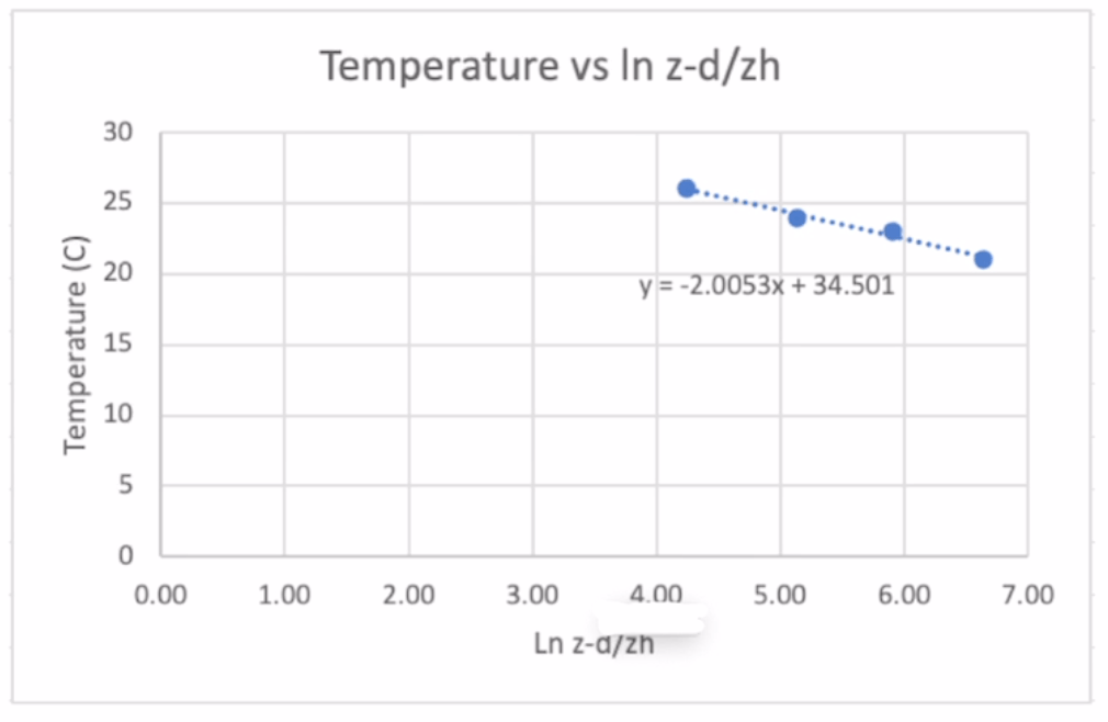
Figure 3 is graphed with the independent variable on the x axis and height on the y axis. If we fit this curve with today’s calculators, it would be fairly easy to get a curve that would fit that. But since it’s a linear equation, we can take the temperature data from Table 1 and the In ((Z-d)/ZH) data from Table 1 and graph them together.
Figure 4. Relationship between temperature and In Z-d/zh
Figure 4 is a graph that shows what happens when we do that. Notice that, just like we suggested, it creates a linear equation (Equation 4).
Equation 4
We learned in Figure 1 the B value was equal to t0 (our aerodynamic surface temperature). Since we know our surface temperature is 34.5 degrees, we can estimate what the temperature is down here at the surface, even though we only measured down 0.2 m.
We also know from Equation 4 that our M value is equal to -2.01. And if we look at Equation 1, our slope value is below.
Equation 5 (the slope value from Equation 1)
So we can write
Equation 6
How to estimate sensible heat flux
Now, if we were interested in the sensible heat flux, which we often are, we can simply rearrange this equation to be
Equation 7
And in Figure 1, I forgot to give you this value, but for an air temperature of 20 degrees celsius,
Equation 8
And then finally, a typical unit for friction velocity, which should be measured in the field over the specific canopy you are in, is about 0.2 meters per second.
Equation 9
So if we did this calculation, we would learned that there’s about 193 watts per meter squared of sensible heat flux coming off that surface.
Equation 10
So if we can measure temperature at a few heights, we can estimate what the heat flux is coming off the surface assuming we know something about our canopy. Learn more about measuring and modeling environmental parameters at metergroup.com/environment. If you have any questions feel free to email Dr. Campbell at [email protected].
What was the life of a scientist like before modern measurement techniques? In our latest podcast, Campbell Scientific’s Ed Swiatek and METER’s Dr. Gaylon Campbell discuss their association with three pioneers of environmental measurement.
Learn what it was like to practice science on the cutting edge. Discover the creative lengths they went to and what crazy things they cobbled together to get the measurements they needed.
The environment plays a large role in any plant study. Ensuring you’re capturing weather and other environmental parameters in the best way allows you to draw better conclusions. To accurately assess plant stress tolerance, you must first characterize all environmental stressors. And you can’t do that if you’re only looking at above-ground weather data.
For example, drought studies are notoriously difficult to replicate and quantify. Knowing what kind of soil moisture data to capture can help you quantify drought, allowing you to accurately compare data from different years and sites.
Get better, more accurate conclusions
It’s important for your environmental data to accurately represent the environment of your site. That means not only capturing the right parameters but choosing the right tools to capture them. In this 30-minute webinar, application expert Holly Lane discusses how to improve your current data and what data you may not be collecting that will optimize and improve the quality of your plant study. Find out:
How to know if you’re asking the right questions
Are you using the right atmospheric measurements? And are you measuring weather in the right location?
Which type of soil moisture data is right for the goals of your research or variety trial
How to improve your drought study, why precipitation data is not enough, and why you don’t need to be a soil scientist to leverage soil data
How to use soil water potential
How accurate your equipment should be for good estimates
Key concepts to keep in mind when designing a plant study in the field
What ancillary data you should be collecting to achieve your goals
Holly Lane has a BS in agricultural biotechnology from Washington State University and an MS in plant breeding from Texas A&M, where she focused on phenomics work in maize. She has a broad range of experience with both fundamental and applied research in agriculture and worked in both the public and private sectors on sustainability and science advocacy projects. Through the tri-societies, she advocated for agricultural research funding in DC. Currently, Holly is an application expert and inside sales consultant with METER Environment.
Everybody measures soil water content because it’s easy. But if you’re only measuring water content, you may be blind to what your plants are really experiencing.
Soil moisture is more complex than estimating how much water is used by vegetation and how much needs to be replaced. If you’re thinking about it that way, you’re only seeing half the picture. You’re assuming you know what the right level of water should be—and that’s extremely difficult using only a water content sensor.
Get it right every time
Water content is only one side of a critical two-sided coin. To understand when to water or plant water stress, you need to measure both water content and water potential.
In this 30-minute webinar, METER soil physicist, Dr. Colin Campbell, discusses how and why scientists combine both types of sensors for more accurate insights. Discover:
Why the “right water level” is different for every soil type
Why soil surveys aren’t sufficient to type your soil for full and refill points
Why you can’t know what a water content “percentage” means to growing plants
How assumptions made when only measuring water content can reduce crop yield and quality
Water potential fundamentals
How water potential sensors measure “plant comfort” like a thermometer
Why water potential is the only accurate way to measure drought stress
Why visual cues happen too late to prevent plant-water problems
Case studies that show why both water content and water potential are necessary to understand the condition of soil water in your experiment or crop
Dr. Colin Campbell has been a research scientist at METER for 20 years following his Ph.D. at Texas A&M University in Soil Physics. He is currently serving as Vice President of METER Environment. He is also adjunct faculty with the Dept. of Crop and Soil Sciences at Washington State University where he co-teaches Environmental Biophysics, a class he took over from his father, Gaylon, nearly 20 years ago. Dr. Campbell’s early research focused on field-scale measurements of CO2 and water vapor flux but has shifted toward moisture and heat flow instrumentation for the soil-plant-atmosphere continuum.
Soil moisture data analysis is often straightforward, but it can leave you scratching your head with more questions than answers. There’s no substitute for a little experience when looking at surprising soil moisture behavior.
Join Dr. Colin Campbell April 21st, 9am PDT as he looks at problematic and surprising soil moisture data.
Understand what’s happening at your site
METER soil scientist, Dr. Colin Campbell has spent nearly 20 years looking at problematic and surprising soil moisture data. In this 30-minute webinar, he discusses what to expect in different soil, environmental, and site situations and how to interpret that data effectively. Learn about:
Telltale sensor behavior in different soil types (coarse vs. fine, clay vs. sand)
Possible causes of smaller than expected changes in water content
Factors that may cause unexpected jumps and drops in the data
What happens to dielectric sensors when soil freezes and other odd phenomena
Surprising situations and how to interpret them
Undiagnosed problems that affect plant-available water or water movement
Why sensors in the same field or same profile don’t agree