Everybody measures soil water content because it’s easy. But if you’re only measuring water content, you may be blind to what your plants are really experiencing. To understand when to water or plant water stress, you need to measure both water content AND water potential.
Learn more in our soil moisture master class, “Secrets of water in soil“. Six short videos teach you everything you need to know about soil water content and soil water potential—and why you should measure them together. Plus, master the basics of soil hydraulic conductivity.
In baseball, the aerodynamic properties of the ball are critical. Pitchers rely on the ball to have a certain amount of lift so it can move in the air to the left or right based on how they throw a curveball.
Did something change on the surface of the ball that allowed more home runs?
The ball can also speed up or slow down based on the amount of drag, or how much the air is resisting the ball’s movement. Because of this, federations such as Major League Baseball want to ensure the ball doesn’t change from year to year. In the past couple of years, a spike in home runs prompted the Major League Baseball federation to contract Washington State University sports science laboratory to help them better understand the aerodynamics of the ball. They want to know: did something change on the surface of the ball that allowed more home runs to be hit?
Tiny changes cause big problems
Even the slightest change in the surface of the ball, such as the seam height or the seam width, can have a large effect on the carry distance of the ball. Jeff Kensrud, assistant director of the WSU Sport Science Lab says, “These balls sometimes hit the wall 350 feet in the outfield, and if that ball would have travelled five more feet, it would have gone over the fence. That’s why we’re trying to quantify the aerodynamic properties of the ball so professional organizations can tell how far the balls are going to travel in the air when they’re hit.”
Kensrud says they have two experiments set up in the lab. One is an environmentally controlled chamber where they do all the bat and ball testing. He says, “We have to maintain 72 ℉ and 50% relative humidity 24 hours, 7 days a week because balls and bats change with temperature and humidity.” The second experiment is an aerodynamic test lab where temperature and humidity are more challenging to control. They need to understand what the microclimate is because weather variables like temperature and barometric pressure are constantly changing, which can affect their calculations.
The ATMOS 14 sensor measures temperature, RH, barometric pressure and vapor pressure
To monitor these parameters, the team uses ATMOS 14 temp/barometric pressure/vapor pressure/and relative humidity sensors and a ZL6 data logger to get near-real-time feedback of what’s going on in their Aero Testing Lab. Kensrud says, “Essentially, we have three sensors hooked up to the ZL6 logger at the beginning, the middle, and the end of our aerodynamic test tunnel. Every half hour, we’ll check ZENTRA Cloud software and put that data directly into our computer so we have the most up-to-date weather information to ensure we’re running our aerodynamic experiment correctly. The tunnel is 60 ft long, so we need to know if the temperature is the same throughout our testing station. A slight change in barometric pressure could alter our calculated coefficient of drag. Sometimes in a matter of a few hours a storm can roll in. And if we are checking that sensor regularly, then we can see drift in our coefficient of drag and we know it had nothing to do with the ball. It’s just the barometric pressure in the city of Pullman changed.”
How tests are run
To test the aerodynamic properties of the balls, the team projects balls into still air at up to 100 miles an hour. They then determine what the coefficient of drag and lift is, or how the balls behave in the airflow. And the team also tests bats.
Researchers measure bat performance using real baseballs
Kensrud says, “For 15 years, we’ve been the exclusive certification center for testing and certifying baseball bats for USA baseball, USA softball, NCAA baseball and most of the amateur baseball world. If you want to certify your equipment for play, it’s going to come through our lab.” For bat testing, researchers measure bat performance using real baseballs. The lab uses pneumatic air cannons that accelerate the ball from at rest up to about 140 miles an hour. The balls are released from the cannon and then impact the bat. Kensrud says, “It’s as close as we can get in a laboratory to a real bat/ball collision on the field.”
Sensors help maintain proper test conditions
Kensrud says using the ATMOS 14 confirmed their hypothesis that there was sometimes a change in temperature over 60 feet in their concrete building where tests are performed. He says, “These sensors are constantly telling us if we have a temperature gradient and how severe it is. If you start out at 75 degrees at the beginning of the tunnel, but by the time you get to the end you’re at 82 degrees, that could be a problem. Especially when you assume your temperature is constant. These sensors help properly monitor the temperature throughout the space and also give a very accurate barometric pressure reading in near-real time. That’s critical for what we’re doing because in this area we can get big storms coming in and out that can affect our measurements. If we have a change in barometric pressure or a temperature gradient of more than two degrees from the beginning to the end, we shut testing down to allow the space to acclimate. The data enables us to set up a go/no go approach to aerodynamic testing.”
Why ball aerodynamics matter
Kensrud says that this research is important to keep the ball constant.
Ball aerodynamics affect both pitching and hitting.
He says, “Some federations need to know when or if the ball has changed. Ball aerodynamics affect both pitching and hitting. The more precise our instruments are in monitoring, the more accurate the results are that we give to these Federations so they can make informed policy decisions on what to do with the ball, or how to keep the ball in spec for years to come.”
What’s the future of aerodynamic sports testing?
Kensrud says he’d love to continue testing for federations like Major League Baseball, but it would be fun to grow and expand into measuring the aerodynamics of other sports balls. He adds, “It’s a bit of a stretch, but it wouldn’t be impossible to think that one day we could be making some high-speed, in-flight, aerodynamic measurements for say, the aerospace industry. But that’s not a contract. That’s me putting my ‘future cap’ on.”
You can learn more about WSU sports science lab testing here.
Soil moisture data are useful, but they can’t tell you everything. Other strategies for growers and researchers, like plant and weather monitoring, can inform water management decisions.
In this webinar, world-renowned soil physicist, Dr. Gaylon Campbell shares his newest insights and explores options for water management beyond soil moisture. Learn the why and how of scheduling irrigation using plant or atmospheric measurements. Understand canopy temperature and its role in detecting water stress in crops. Plus, discover when plant water information is necessary and which measurement(s) to use. Find out:
Why the Penman-Monteith equation, with the FAO 56 procedures, gives a solid, physics-based method for determining potential evapotranspiration of a crop
How the ATMOS 41 microenvironment monitor combined with the ZL6 logger and ZENTRA Cloud give easy access to crop ET data
How assimilate partitioning can be controlled by manipulating plant water potential using appropriate irrigation strategies
Why combining monitoring soil water potential with deficit irrigation based on ET estimates provide an efficient and precise method for controlled water stress management
Dr. Gaylon S. Campbell has been a research scientist and engineer at METER for over 20 years, following nearly 30 years on faculty at Washington State University. Dr. Campbell’s first experience with environmental measurement came in the lab of Sterling Taylor at Utah State University making water potential measurements to understand plant water status.
Dr. Campbell is one of the world’s foremost authorities on physical measurements in the soil-plant-atmosphere continuum. His book written with Dr. John Norman on Environmental Biophysics provides a critical foundation for anyone interested in understanding the physics of the natural world. Dr. Campbell has written three books, over 100 refereed journal articles and book chapters, and has several patents.
If you’re not using an accurate weather station at your field site to gather data for growing degree day (GDD) or thermal time calculations, you should start now.
GDD predictions save you hours of scouting time and can increase yield because they’re a scientific way to know the best time for insect/disease control measures. In this chalk talk, Dr. Colin Campbell explains the concept of thermal time (or growing degree days) and shows two different ways to calculate it.
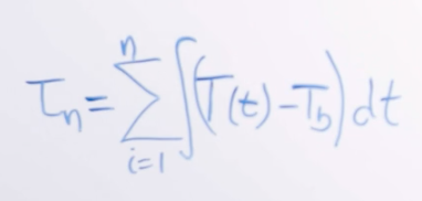
Hello, my name is Dr. Colin Campbell. I’m a senior research scientist here at METER Group. Today, we’re going to give a brief primer on thermal time. When I talked to some of my colleagues about that, they mentioned that thermal time (or growing degree days) is really just a way to match a plant’s clock with our clock. It helps us understand what’s happening with the plant, and we can predict things like emergence, maturity, etc. And the way we do this is through this equation that is pretty simple (Equation 1).
Equation 1
We can sum thermal time (Tn) by taking the summation of day one to day n of the average temperature (meaning T max plus T min divided by two), minus a base temperature (Tbase), and then multiply by time step (delta t). And in this case, our time step is just one day.
So the whole analysis is simply the average temperature minus a base temperature. We get that value each day. And then we keep summing until it reaches a value that tells us that we’ve progressed from one stage to another stage.
A good example of this is wheat. When I was young, I did an experiment on this in biology. The idea was that for emergence, the wheat plant needs 78 day degrees from planting to emergence. So I used Equation 1, and when I had summed enough day degrees, I knew the wheat was moving from the planting stage to a post emergent stage. I went out and measured the wheat and it actually matched up well. Not every wheat plant emerged at that point, but the average was quite close.
So what does that mean in terms of graphical data? I wanted to show you what this equation actually looked like and then plant a seed in your mind for our next discussion, which will be, how good is this analysis? If you think about modern technology, like the ATMOS 41 weather station, you can get temperature measurements that are every five minutes or even every one minute. So wouldn’t it be better if we collected our thermal time information with this equation (Equation 2)?
Equation 2
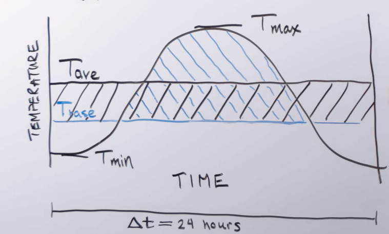
We can take the sum over each day, like we did in Equation 1, but instead we take the integral of temperature at a small time step T(t) (like five minutes) minus the base temperature (Tb) and then just integrate this across the day. We’re going to learn about that in my next chalk talk. But for now, let’s go to this graph (Figure 1).
Figure 1. Temperature vs. time over 24 hours
In Figure 1, we have temperature on the y axis and time on the x axis. The total time is 24 hours. This is our daily step, where we’re collecting this information about thermal time. And here are all the parameters from the equation: the maximum temperature (Tmax), the minimum temperature (Tmin), and the average temperature (Tave). And then this is a base temperature (Tbase). And to familiarize you with what we’re talking about, Tbase is the temperature below which progress is not made in the development of this plant. The progress is not reversed, meaning if it’s below the base temperature, the plant is not reversing its development, but it just doesn’t progress.
The black line is what I’ve drawn as a typical diurnal temperature swing. So it’s going from a minimum in the early morning up to a maximum sometime in the afternoon. And I’ve tried to compare these two approaches. One one side, we have the average temperature and the base temperature. This rectangle is our thermal time for that day. But the question is, with all our temperature data (like from the ATMOS 41) where we have pretty small time increments, could we instead just integrate over the day and then collect all the information on thermal time that is below this black line (the actual temperature, and of course, we subtract out the base temperature). How much difference does that make compared to this here? And what are the implications of not being able to measure our temperature terribly accurately? We’re going to talk about that in our next discussion, and I look forward to seeing you then.
Take our Soil Moisture Master Class
Six short videos teach you everything you need to know about soil water content and soil water potential—and why you should measure them together. Plus, master the basics of soil hydraulic conductivity.
Measuring soil hydraulic properties like hydraulic conductivity and soil water retention curves is difficult to do correctly. Measurements are affected by spatial variability, land use, sample prep, and more.
Leo Rivera teaches soil hydraulic properties measurement best practices
Getting the right number is like building a house of cards. If one thing goes wrong—you wind up with measurements that don’t truly represent field conditions. Once your data are skewed in the wrong direction, your predictions are off, and erroneous recommendations or decisions could end up costing you a ton of time and money.
Get the right numbers—every time
For 10 years, METER research scientist, Leo Rivera, has helped thousands of customers make saturated and unsaturated hydraulic conductivity measurements and retention curves to accurately understand their unique soil hydraulic properties. In this 30-minute webinar, he’ll explain common mistakes to avoid and best practices that will save you time, increase your accuracy, and prevent problems that could reduce the quality of your data. Learn:
Sample collection best practices
Where to make your measurements
How many measurements you need
Field mapping tools
How to get more out of your instruments
How to use the LABROS suite to fully characterize soils (i.e., full retention curves and hydraulic conductivity curves)
Best practices for measuring field hydraulic conductivity using SATURO
In this chalk talk, METER Group research scientist, Dr. Colin Campbell, extends his discussion on humidity by discussing how to calculate vapor pressure from wet bulb temperature. Today’s researchers usually measure vapor pressure or relative humidity from a capacitance-based relative humidity sensor.
However, scientists still talk in terms of wet bulb and dew point temperature. Thus, it’s important to understand how to calculate vapor pressure from those variables.
Hello, my name is Dr. Colin Campbell. I’m a research scientist here at METER group, and also an adjunct professor at Washington State University where I teach a class on environmental biophysics. And today we’re going to be extending our discussion on humidity by talking about how using a couple of common terms related to humidity, we can calculate vapor pressure. The first term we’re going to talk about is dew point temperature. I’ve drawn a couple of figures below that illustrate a test I performed when I was a graduate student in a class related to biophysics.
Dew Point Temperature Test Illustration
The professor had us take a beaker of water and a thermometer and put ice in the beaker and start to stir it. The thermometers were rotating around in the glass, and our job was to look carefully and find out when a thin film of dew began to form around on the glass. So we watched the temperature go down, and at some point, we observed a thin film form onto that glass. At the point the film began to form, we looked at the temperature to get the dew point temperature, which means exactly what it says: the point at which dew begins to form.
This experiment wasn’t perfect because there is certainly a temperature difference between the inside of our glass where we’re stirring with the thermometer and the outer surface of the glass. But it was a good approximation and a great way to demonstrate what dew point temperature is. So we can say that the dew point temperature is the point at which the air is saturated and water begins to condense out. We call this Td or dew point temperature. The beautiful thing about dew point temperature is that if you know this value, you can easily calculate vapor pressure and even go on to calculate relative humidity, as I talked about in another lecture.
To calculate vapor pressure from our dew point temperature, we’ll call vapor pressure of the air, ea which is equal to the saturation vapor pressure (es) at the dew point temperature (Td) (Equation 1).
Equation 1
And as I discussed in my other lecture, the saturation vapor pressure is a function of the temperature (not multiplied by the temperature). It’s pretty simple to get the saturation vapor pressure at the dew point temperature. We simply use Tetons formula (Equation 2 discussed here), which says that the saturation vapor pressure at the dew point is equal to 0.611 kilopascals times the exponential of b Td over C plus Td (Td being the dewpoint temperature).
Equation 2
So let’s assume our dew point temperature is five degrees C. This is something you can find in many weather reports. If you look down the list of measurements carefully, it’s usually there. So the vapor pressure of the air (ea) is calculated by the formula I showed (Equation 1). Our first constant b is 17.502 and our second constant C, is just 240.97 degrees C. If we plug all the values into that equation, it ends up that our vapor pressure is 0.87 kilopascals.
Equations 3 a, b, and c
Now there might be a variety of reasons we want this value. We might want to use it to calculate the relative humidity. If so, we’d simply divide that by the saturation vapor pressure at the air temperature. Then we’d have our relative humidity. More commonly we use the ea and the saturation vapor pressure at the air temperature to calculate the vapor deficit. So possibly in some agronomic application that might be interesting to us. So that is dew point temperature.
Now we’ll talk about another common measurement, our wet bulb temperature. This was much more common in past years where there weren’t electronic means to measure things like dew point or humidity sensors. And we used to have to make a measurement of humidity by hand. And what they did was to collect a dry bulb temperature or a standard air temperature. And that dry bulb temperature (or the temperature of the air) was compared to what we call a wet bulb temperature.
Wet Bulb Temperature
Researchers made this wet bulb temperature by putting a cotton wick around the bulb of the thermometer. This was just a fabric with water dripped onto it. Once that wick is saturated with water, the water begins to evaporate, and they would use wind to enhance that evaporation. For example, some instruments had a small fan inside that would blow water across this wick, or more commonly, two temperature sensors were attached on a rotating handle, so they could spin them in the air at about one meter per second (or two miles an hour). I don’t know how you’d ever estimate that speed, but that was the goal. This would help the water evaporate at an optimum level.
You can imagine what happens during this evaporation by thinking about climbing out of the pool. You feel some cooling on your skin as water begins to evaporate when you climb out of a pool on a dry, warm summer day. That’s water as it changes from liquid into water vapor, and it actually takes energy for this to happen (44 kilojoules per mole). That’s actually quite a bit of energy used for changing liquid water into water vapor. When that happens, it decreases the temperature of this bulb. If we wait till we’ve reached that maximum temperature decrease, we can take that as our wet bulb temperature, or Tw.
This wet bulb temperature is not quite as simple as our dew point temperature to use in a calculation. Here’s the calculation we need to estimate vapor pressure from the wet bulb temperature.
Equation 4
We take the saturation vapor pressure (es) at the wet bulb temperature (Tw) and subtract, the gamma (Ɣ), which is the psychrometer constant 6.66 times 10-4 ℃-1 times the pressure of the air (Pa), multiplied by the difference between the air temperature (Ta) or that dry bulb that I mentioned earlier, and the wet bulb temperature (Tw).
Gamma is an interesting number. It’s actually the specific heat of air divided by the latent heat of vaporization, or that 44 kilojoules per mole that I mentioned before. We can simply take it as a constant for our purposes here as 6.66 times 10-4 ℃-1. So let’s actually put it into a calculation. Our example problem says find the vapor pressure of the air. If air temperature (Ta) is 20 degrees Celsius, the wet bulb temperature (Tw) is 11 degrees Celsius, and air pressure (Pa) is 100 kilopascals (basically at sea level). And just to remind us, this is the constant gamma (6.66 times 10-4 ℃-1). Air pressure is 100 kilopascals. We take this standard equation (Equation 4) and insert all these numbers.
Equation 5
So our vapor pressure is going to be this calculation from Tetons formula (Equation 2) and if you plug all those numbers into your calculator (notice our degrees C will cancel) we’re left with kilopascals. So our vapor pressure is about 0.71 kilopascals. So that is how we calculate the vapor pressure from the wet bulb temperature.
I hope this has been interesting. These are values that you may hear about. It’s less common today since we usually get our relative humidity from a capacitance-based relative humidity sensor, but still scientists talk in terms of wet bulb and dew point temperature. So it’s important to understand how we actually calculate our vapor pressure from those variables. If you’d like to know more about this, please visit our website, metergroup.com, and look at some of the instruments that are there to make measurements. Or you can email me if you want to know more at [email protected]. I hope you have a great day.
Hypoxic floods can be catastrophic for river ecosystems, often leading to widespread fish kills or other alterations in fish community composition and behavior. Hypoxia in rivers is uncommon due to the high rates of re-aeration in flowing waters, and when it does occur, it’s typically associated with human pollution (high nutrient loading). However, in the East African Mara River, hypoxic flooding events are not caused by humans, but by hippos.
Hippopotamia in East African Mara River
Over the past ten years, Dr. Christopher Dutton, aquatic ecologist at Yale University, and other researchers have documented frequent hypoxic floods and fish kills in the Mara river system. He says, “Our research shows these floods are caused by the flushing of hippopotamus pools. There are over 4000 hippopotami in the Kenyan portion of the Mara River bringing in over 3500 kg of organic carbon into the aquatic ecosystem each day. Hippo pools within the three tributaries of the Mara become anoxic under low discharge, while increases in discharge flush out the hippo pools and carry a hypoxic pulse of water through the river downstream.”
Hippopotamus Pool on the Mara River
Dutton and his team aim to understand the drivers of variability in these hypoxic floods and how these floods are propagated downstream in order to predict how the frequency and intensity of these events will be influenced by climate and land use change.
Unexpected patterns in dissolved oxygen
Dutton says they first noticed unusual patterns in aquatic health while working on another project. “When we started working in Kenya, we were trying to determine the environmental flows needed to maintain proper ecosystem function. We sampled from up in the forest down through the protected areas in the Masaai Mara and the Serengeti. We found the traditional indicators of water quality started to get much worse in the protected areas. This was surprising to us because we assumed water flowing through a protected area would be getting cleaner. But after we collected enough data, we could see that dissolved oxygen was crashing on average every 12 days for 8 to 12 hours and then rebounding. We hadn’t seen that in other rivers. This drew us to wonder if it was being caused by the flushing of hippo pools.”
Dutton says hippopotamus pools are slack water areas on the main river channel where hippos gather throughout the day because they don’t like fast moving water. He explains, “Every day they lounge in the water because their skin is sensitive to UV and gets desiccated in the sun. But at night and in the early morning, they leave the pools, go to the grassland, and eat tons and tons of grass. Afterward, they go back to the pool to rest, sleep, and defecate. They defecate so much organic matter into the river, it alters aquatic metabolism in ways that haven’t yet been fully understood.”
Hippopotamia Gathering in a Hippopotamus Pool
Dutton wants to understand how the organic matter and inorganic nutrients the hippos bring in are altering the ecosystem and what’s causing variability in the degree of hypoxia.
What’s causing the variability?
Dutton thinks there are two likely drivers of hypoxia: time since hippo pools were flushed and the size of the rainfall driving the event. He says, “Because rainfall in the Mara region is highly localized within and among catchments, the biogeochemistry that causes hypoxia can vary among pools and tributaries. Understanding these dynamics requires fine scale spatial and temporal data on precipitation patterns across the catchment.”
Dutton is using ATMOS 41 weather stations and METER data loggers in three Mara sub catchments to monitor the intensity and frequency of rainfall during these episodic floods where rains can be highly variable in space. He’s also documenting hippo pool biogeochemistry along with discharge and dissolved oxygen (DO) response in the main stem and tributaries. He’s using a water quality sonde to monitor DO and turbidity. He says, “We’re trying to quantify these events in the various catchments because they are different geologically. One of them has more sulfur containing rocks which causes sulfates in the water. In a reducing environment, sulfates turn into hydrogen sulfide which is toxic to fish. So we’re trying to parse out what’s really killing the fish in these different catchments.”
He says the data show there is such high biochemical oxygen demand from the bottom of these pools, that when the organic waste and reduced compounds are flushed, they continue to suck oxygen out of the river as the waste moves downstream. This often causes fish kills in the river. He adds, “We’ve seen thousands of fish dead after one of these events. But interestingly, the next day, it’s like it never happened. There are no fish anywhere on the bank. They’ve already been consumed by hyena, vultures, marabou, storks, and even lions.”
Data collection challenges
Dutton says collecting precipitation data in East Africa has unusual challenges. He says, “One of our sites is close to a hyena den. They occasionally go and unplug wires. And one of our weather stations was taken by an elephant. I concreted it in, but the elephant took it and dropped it 100 meters away.”
The team avoids losing data by locating their measurement stations near tourist camps, where locals can watch over the equipment. Dutton says, “We build fences around each of the stations, and we concrete them into the ground, but our biggest strategy is putting the site close to a camp. The Kenyans that run the camps are excited to have a weather station nearby. They enjoy seeing the data and sharing it with their guests.”
The team builds fences around installations to protect them from hyenas and other animals
What’s the future of the research?
Dutton says the team is still working on collecting data, which is not always easy. He says, “This year, a 100-year flood occurred in the Mara which destroyed our water quality sonde. The water got so high the compression on the sonde popped out all the sensors. We lost two months of data. So we haven’t yet been able to look closely at the relationships between the rainfall, the different catchments, and these crashes, but that’s something we’ll do as soon as we can get to the data.”
He says this research is important because the Mara River system is still a natural river system essentially untouched by humans with much of its megafauna intact, which is rare. He adds, “The hippos are a very natural part of this river, and these processes we’re documenting help us understand how rivers may have functioned prior to the removal of larger megafauna. In the last 50 years, there has been large scale deforestation in the upper catchment. Some people speculate that this is causing more erratic flows. So what happens when the flows become more (or less) than normal?”
Dutton recently published a peer-reviewed paper on the detailed biogeochemistry of the hippo pools in Ecosystems Journal. You can read it here. And you can read the team’s first paper documenting these events published on nature.com here.
If you rely on soil moisture data to make decisions, understand treatment effects, or make predictions, then you need that data to be accurate and reliable. But even one small oversight, such as poor installation, can compromise accuracy by up to +/-10%. How can you ensure your data represent what’s really happening at your site?
Chris Chambers discusses how people unknowingly compromise their soil moisture data.
Best practices you need to know
Over the past 10 years, METER soil moisture expert Chris Chambers has pretty much seen it all. In this 30-minute webinar, he’ll discuss 6 common ways people unknowingly compromise their data and important best practices for higher-quality data that won’t cause you future headaches. Learn:
Are you choosing the right type of sensor or measurement for your particular needs?
Are you sampling in the right place?
Why you must understand your soil type
How to choose the right number of sensors to deal with variability
At what depths you should install sensors
Common installation mistakes and best practices
Soil-specific calibration considerations
How cable management can make or break a study
Factors impacting soil moisture you should always record as metadata
Choosing the right data management platform for your unique application
If you want accurate data, correct sensor installation should be your number one priority. When measuring in soil, natural variations in density may result in accuracy loss of 2 to 3%, but poor installation can potentially cause accuracy loss of greater than 10%.
Proper sensor installation is the foundation for the data you collect. If you have a poor foundation, it makes data interpretation difficult. In this article, get insider tips on how to install soil moisture sensors faster, better, and for higher accuracy. Learn:
What to be aware of when installing sensors
What installation trouble looks like in your data
Installation priorities for soil moisture sensors
How METER is advancing the science of installation for higher quality data
Understand your sensors
To understand why poor sensor installation has an enormous impact on the quality of your data, you’ll need to understand how soil moisture sensors work.
Soil moisture sensors (water content sensors) measure volumetric water content. Volumetric water content (VWC) is the volume of water divided by the volume of soil (Equation 1) which gives the percentage of water in a soil sample.
Equation 1
So, for instance, if a volume of soil (Figure 1) was made up of the following constituents: 50% soil minerals, 35% water, and 15% air, that soil would have a 35% volumetric water content.
Figure 1. Soil constituents
Why capacitance sensors work
All METER soil moisture sensors use an indirect method called capacitance technology to measure VWC. “Indirect” means a parameter related to VWC is measured, and a calibration is used to convert that amount to VWC. In simple terms, capacitance technology uses two metal electrodes (probes or needles) to measure the charge-storing capacity (or apparent dielectric permittivity) of whatever is between them.
Figure 2. Capacitance sensors use two probes (one with a positive charge and one with a negative charge) to form an electromagnetic field. This allows them to measure the charge-storing capacity of the material between the probes.
Ever spent hours carefully installing your weather station in the field and then come back only to discover you made mistakes that compromised the installation? Or worse, find out months later that you can’t be confident in the quality of your data?
Installing ATMOS 41 Weather Stations
Our scientists have over 100 years of combined experience installing sensors in the field, and we’ve learned a lot about what to do and what not to do during an installation.
Best practices for higher accuracy
Join Dr. Doug Cobos in this 40-minute webinar as he discusses weather station installation considerations and best practices you don’t want to miss. Learn:
General siting and installation best practices
Installation recommendations from WMO and other standards organizations
Common installation mistakes
How to identify installation mistakes in your data
Microclimate variability and how to pick a representative location