Like a silent battle cry, plants call out to signal they are under siege as a warning to other plants and to call in reinforcements to fend off the invasion.
Listen to research on pathogen infection, water stress, and how plants communicate and defend themselves.
How does this communication work? What else are plants doing to protect themselves from disease and predators alike? In our latest podcast, Natalie Aguirre, a PhD candidate and plant physiology and chemical ecology researcher at Texas A&M University, dives into her research on pathogen infection, water stress, and how plants communicate and defend themselves.
Natalie Aguirre graduated with a degree in biology from Pepperdine University, where she completed an honors thesis conducting research on the interaction of drought stress and pathogen infection in chaparral shrubs. She then spent a year as a Fulbright scholar in Spain, studying the effect of water stress on Dutch Elm Disease. Most recently, Natalie worked for the Everglades Foundation, creating educational programs and materials about the Florida Everglades.
The views and opinions expressed in the podcast and on this posting are those of the individual speakers or authors and do not necessarily reflect or represent the views and opinions held by METER.
Abiotic stress in plants: How to assess it the right way
As a plant researcher, you need to effectively assess crop performance, whether you’re selecting the best variety, trying to understand abiotic stress tolerance, studying disease resistance, or determining climate resilience. But if you’re only measuring weather data, you might be missing key performance indicators. Water potential is underutilized by plant researchers in abiotic stress studies even though it is the only way to assess true drought conditions when determining drought tolerance in plants. Learn what water potential is and how it can improve the quality of your plant study.
Soil directly impacts plant growth via nutrient availability, disease pressure, root growth, and water availability.
Quantitative genetics in plant breeding: why you need better data
If you’ve studied plant populations, you’re probably familiar with the simplified equation in Figure 1 that represents how we think about the impact of genetics and the environment on observable phenotypes.
Figure 1. Phenotype = Genotype + Environment
This equation breaks down the observed phenotype (plant height, yield, kernel color, etc.) into the effects from the genotype (the plants underlying genetics) and the effects of the environment (rainfall, average daily temperature, etc.). You can see from this equation that the quality of your study directly depends on the kind of environmental data you collect. Thus, if you’re not measuring the right type of data, the accuracy of your entire study can be compromised.
Water potential: the secret to understanding water stress in plants
Drought studies are notoriously difficult to replicate, quantify, or even design. That’s because there is nothing predictable about drought timing, intensity, or duration, and it’s difficult to make comparisons across sites with different soil types. We also know that looking at precipitation alone, or even volumetric water content, doesn’t adequately describe the drought conditions that are occurring in the soil.
Figure 2. The TEROS 21 is a field sensor used to measure soil water potential
Soil water potential is an essential tool for quantifying drought stress in plant research because it allows you to make quantitative assessments about drought and provides an easy way to compare those results across field sites and over time. Let’s take a closer look to see why.
In this chalk talk video, world-renowned soil physicist, Dr. Gaylon Campbell, discusses how many measurements researchers and growers need to characterize soil moisture at a field or research site. He explores the question: What is the relationship between the measurements that you make and the underlying value of water content in the field?
Presenter
Dr. Gaylon S. Campbell has been a research scientist and engineer at METER for 19 years following nearly 30 years on faculty at Washington State University. Dr. Campbell’s first experience with environmental measurement came in the lab of Sterling Taylor at Utah State University making water potential measurements to understand plant water status. Dr. Campbell is one of the world’s foremost authorities on physical measurements in the soil-plant-atmosphere continuum. His book written with Dr. John Norman on Environmental Biophysics provides a critical foundation for anyone interested in understanding the physics of the natural world. Dr. Campbell has written three books, over 100 refereed journal articles and book chapters, and has several patents.
We quite often get a question from customers about how many measurements we need to characterize soil moisture at a site. And so that’s what I want to talk about today. A number of years ago, I knew a man who was wanting to provide a business of making soil moisture measurements for the purpose of irrigation scheduling for farmers. And he came to me wondering how many samples he should take. He figured that he wanted a fairly simple way of determining soil moisture.
So, he thought he would go into the field and he would collect soil samples from the field, he would take them back to the laboratory, he would dry them and weigh them and dry them and determine water content. And he wondered how many samples would be required to determine the water content to provide this information for a farmer.
Now, that’s not so different from the kinds of information that are often required either for practical applications like irrigation scheduling, or for research purposes. We can see the broader applications of the question of, “what’s the relationship between the measurements that we take and the underlying value of water content in the field?”
Soil water content will vary from place to place.
I think you can see that the same thing would apply whether we were taking samples and bringing them back to the laboratory, or if we were putting in soil moisture sensors, and wanting to monitor soil moisture in the field. So, the first thing we need to talk about soil moisture is a random variable, we need some vocabulary for talking about that. Two terms are important: mean and standard deviation.
If we were to collect many samples of water content from a field, and we were to plot the number of samples versus the water content of the samples, we would obtain a relationship something like this. We would get the most samples around some central value, and that central value is the mean.
The standard deviation is a measure of the dispersion around the mean. 68% of the values that we take would be within plus or minus one standard deviation of that mean value. 95% would be within plus or minus two standard deviations of the mean value.
So, let’s say that we walked out here in the field, and we took a sample and made a measurement on it. And let’s say out of that sample, we determined the water content was 27%. Now let’s say that we assume or we know from some means that the standard deviation is 3%. Then, by these ideas, we would know that the mean value – the expected value for the water content – is or at least there would be a 95% probability that the mean value of the water content would be somewhere between 21% and 33%. The mean value plus two times the standard deviation and the mean value minus two times the standard deviation.
Now we may say, “well that’s not good enough. We need better values than that. So what do we do? We need to take more samples. And so we take a number of samples and average them. And so we can know what the result of averaging several samples is, with a simple relationship. The uncertainty in the average value that we get–the standard deviation of the mean–is the standard deviation, divided by the square root of the number of samples.
So let’s say that we went out in the field, and we took 100 samples. Then the standard deviation of the mean, would be our standard deviation that we assumed before, divided by the square root of 100. The square root of 100, of course, is 10. And so that would be 0.3%. If we determined a value of 28% for that mean of the 100 samples, then with 95% confidence, we can say that the water content is between 27.4 (2 standard deviations below the mean), and 28.6.
Now we’re getting closer then to our quest of determining the number of samples that we need to take. We start out with that equation that we just had that the standard deviation of the mean is equal to the standard deviation divided by the square root of the number of samples. We can rearrange that to say that the number of samples that we need is equal to the standard deviation divided by the standard deviation of the mean, and that value squared. So, the error that we normally would talk about in the measurement–if we’re again talking about 95% confidence–the error is half of the standard deviation of the mean.
This number of samples is two times the standard deviation over the air, and that all squared. So, if we work through a little problem with that, how many samples would we need in order to know the water content within 1%? If the standard deviation is 3%, the way we’ve assumed.
So, the standard deviation is 3%. The error value that we want to get to is 1%. We want to take enough samples so that we have 95% confidence that we’re within 1%. And so the number of samples is 2 times 3%, divided by the air, 1%, and that’s all squared. And that comes out to be 36 samples. Well, when we see that number, typically we get pretty discouraged. That’s more samples than we want to take. More samples probably than we can afford to take.
To see how that relates to reality, we did a little experiment. Here we have a soccer field out behind the METER (formerly Decagon) building. We went out and took one of our sensors, the GS3, and hooked it up to our little handheld device. And we set up three transects 20 meters long, parallel with each other and spaced a meter apart. We went along and took samples every meter along these transects. And I have a little video here that shows how that sampling went. The result of that sampling is shown in this next slide.
This slide shows the result of that set of measurements that we made. And you can see it looks about like you would expect it to. We’ve got some variation, we show a mean value and some variation around it. The transects, again, showed variability but seemed to be showing about the same result for each transect. We had 60 samples there.
The average water content that we computed was 38.6%. The standard deviation was not 3%, but 5%. So, the situation is even worse than we imagined with these calculations that we just did here. With a standard deviation of 5%, if we want to know the water content within 1%, we would need 100 samples to do that. And so even with our 60 samples, here, our standard deviation of the mean is 0.65%. And so our field water content is somewhere between 37.3 and 39.9.
Well, as I say that usually is discouraging when we get to that point and see how many samples are needed to make a set of measurements, but the thing is that quite often, the thing that we need to know is not an accurate value for the average water content. Quite often, what we want to know is how much the water content is changing. And that we can know in other ways, accurately enough, so that we don’t need that many samples.
That person that I started out talking about who was wanting to schedule irrigation would need to know water content with an accuracy of 1%. Well, at least with a precision of 1% or better. But that could be achieved much more readily by installing a sensor in situ, where you’re not dealing with the spatial variability in the soil and monitoring that.
Here I’ve shown some data that we took in the field with one of our 5TE sensors hooked up to a data logger. The water content is sampled every minute, it’s averaged over hour intervals, and the plot that you see here is a plot of the water content measured each hour. Then, you can see a period of time where the soil is drying, because the plants are using water. You can see an increase in water content that results from adding water through irrigation or rain. And then again, the water content decreasing as the water is used. And you see very little variation in those data.
Now if this guy that wanted to provide the irrigation scheduling service, had wanted to do this same thing by sampling, the next slide shows the result that he would have gotten if he had gone out every hour and taken one soil sample and plotted the result.
This is what he would have gotten; the blue lines that you see. And you can see that it’s about what you would expect: that the highest values are about 10% higher than the mean value, the lowest values are about 10% lower, and the standard deviation we said is about 5. So, that’s about what we would expect. But from these kinds of data, there’s no possibility that you could ever tell when you should irrigate.
In the next slide, I show the result that you would have gotten if you went out and took 10 samples every hour. And here you can see the pattern to some extent of when the drying and wetting occur, but there’s still an awful lot of variation.
The next slide shows the result of taking 100 samples every hour, a ridiculous thought, but again, there’s still some variation in it. It still doesn’t look anywhere near as good as the in situ sample. When we’re just looking for the changes in water content, the water storage, and water use, in situ measurements make a lot more sense than soil moisture sampling.
So, let me conclude just by a few points that I hope to have made in this. First of all, the soil water content varies from place to place; that’s inherent in nature. It’s something that we expect anytime we go out to measure soil moisture. We usually need to take an average of moisture at several locations in order to know what the water content of a field is, or an experimental site. We usually can’t afford to take enough measurements to really know what it is to have it within the accuracy that we would like to have it. And so we can go through this exercise that I’ve gone through here, we can determine the number that we need, but usually, our budget won’t allow us to put in that many and so we end up compromising to some extent.
In our latest podcast, Dr. Cristine Morgan, one of the US’s premier soil scientists and Chief Scientific Officer at the Soil Health Institute shares her views on soil health: what it is, how to quantify it, what’s the payoff, and why it’s so critical to our success as a society.
“Our soils support 95 percent of all food production, and by 2060, our soils will be asked to give us as much food as we have consumed in the last 500 years.” (Credit: https://livingsoilfilm.com/)
Her thoughts? “We all live or die by soil, literally. We just have to remind people that it’s about quality of life. It’s about the food that you eat. It’s about the safety and welfare of your children.”
Dr. Cristine Morgan is the Chief Scientific Officer at the Soil Health Institute in North Carolina. Learn more about the Soil Health Institute on their website.
The views and opinions expressed in the podcast and on this posting are those of the individual speakers or authors and do not necessarily reflect or represent the views and opinions held by METER.
In his latest chalk talk, Dr. Colin Campbell, environmental scientist at METER Group, teaches how to model vertical variation in temperature and how to estimate sensible heat flux.
Video transcript
Hello, everyone. My name is Dr. Colin Campbell, and I’m a senior research scientist here at METER Group. For today’s chalk talk, we’ll be talking about modeling vertical variation in temperature. In Figure 1, I’ve put together a graph that shows the maximum and minimum temperature with height and depth in the soil at some snapshot in time at a particular place.
Figure 1. Maximum and minimum temperature with height and depth at a snapshot in time, in a particular place
It’s interesting to note that the change in temperature with depth in the soil is much faster than the change in temperature with height, whether we’re talking about a maximum or minimum. And the reason is that even though air is a good insulator, it also mixes really well. And that mixing is caused by eddies. And there’s a little more to that story. It depends specifically on surface heating by the sun through radiation and the cover type, whether it’s plants, rocks, boulders, straight soil, snow, or wind.
Equation 1
If we were going to model that, we would start by writing an equation (Equation 1) where a temperature at sun height, Z, above the surface (see variables noted in Figure 1), is equal to an aerodynamic surface temperature, T0, minus the sensible heat flux, divided by 0.4 times rho, CP, which is the volume specific heat of the air, times a variable called u*, which is the friction velocity. We multiply all that by the logarithm of z, the height above the surface minus d, which is the zero plane displacement, divided by z h, which is a roughness parameter. You might notice up here in the list of variables, that the zero plane displacement is 0.6 times H. H is the canopy height in meters. The rough roughness parameter can be estimated as 0.02 times the canopy height or times H. Now we have an equation that will help us model temperature with height.
However, often we don’t know things like H, our sensible heat flux, and u*, our friction velocity. One of the things that we notice about this equation is that it’s set up somewhat like a linear equation. As you know, an example of a linear equation is something like Equation 2.
Equation 2
Figure 1 isn’t written quite that way, but if we look closely at the example below (Equation 3), this value could be our b, and this value our m, and this value could be our x. And if we do that, we actually can get some use out of graphing temperature with height.
Equation 3
So we went out one day and measured this with a METER Group set of environmental sensors set up at certain heights above the surface. Here we placed sensors at 0.2 m, 0.4 m, 0.8 m, and 1.6 m above the ground.
Table 1
To visualize this, in Figure 2 we graphed height on the y axis and temperature on the x axis, similar to the graph in Figure 1.
Figure 2. Graph showing the relationship between height and temperature
We know from Equation 1 that the axes for temperature and height should be switched because temperature is the dependent variable, and height is the independent variable. So if we switch axes it would look like the graph in Figure 3.
Figure 3. Graph showing the relationship between height and temperature where temperature is the dependent variable and height is the independent variable.
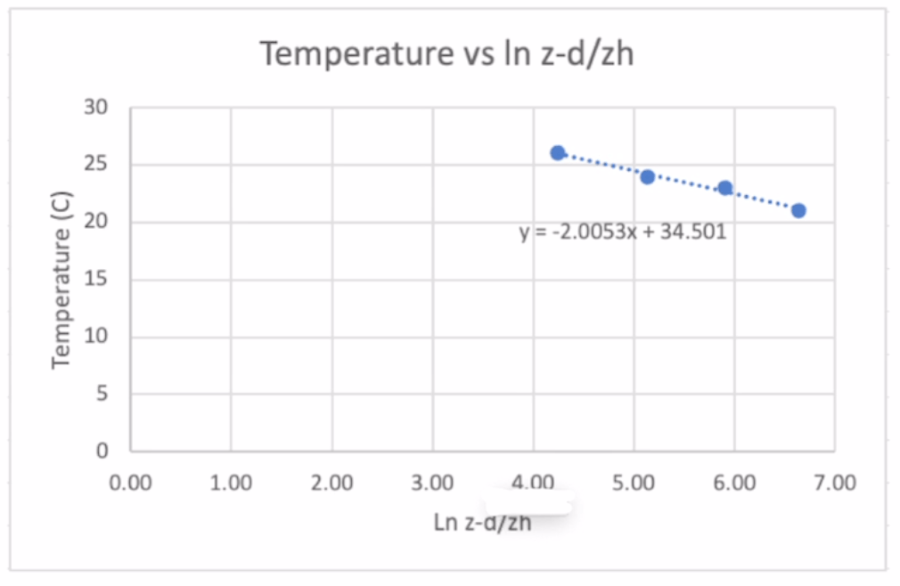
Figure 3 is graphed with the independent variable on the x axis and height on the y axis. If we fit this curve with today’s calculators, it would be fairly easy to get a curve that would fit that. But since it’s a linear equation, we can take the temperature data from Table 1 and the In ((Z-d)/ZH) data from Table 1 and graph them together.
Figure 4. Relationship between temperature and In Z-d/zh
Figure 4 is a graph that shows what happens when we do that. Notice that, just like we suggested, it creates a linear equation (Equation 4).
Equation 4
We learned in Figure 1 the B value was equal to t0 (our aerodynamic surface temperature). Since we know our surface temperature is 34.5 degrees, we can estimate what the temperature is down here at the surface, even though we only measured down 0.2 m.
We also know from Equation 4 that our M value is equal to -2.01. And if we look at Equation 1, our slope value is below.
Equation 5 (the slope value from Equation 1)
So we can write
Equation 6
How to estimate sensible heat flux
Now, if we were interested in the sensible heat flux, which we often are, we can simply rearrange this equation to be
Equation 7
And in Figure 1, I forgot to give you this value, but for an air temperature of 20 degrees celsius,
Equation 8
And then finally, a typical unit for friction velocity, which should be measured in the field over the specific canopy you are in, is about 0.2 meters per second.
Equation 9
So if we did this calculation, we would learned that there’s about 193 watts per meter squared of sensible heat flux coming off that surface.
Equation 10
So if we can measure temperature at a few heights, we can estimate what the heat flux is coming off the surface assuming we know something about our canopy. Learn more about measuring and modeling environmental parameters at metergroup.com/environment. If you have any questions feel free to email Dr. Campbell at [email protected].
In our latest podcast, Dr. Neil Hansen, BYU professor of environmental science, discusses water conservation, the latest research on getting more crop per drop, exciting applications of remote sensing, and the challenges we face trying to meet changing water demands in a growing population.
The views and opinions expressed in the podcast and on this posting are those of the individual speakers or authors and do not necessarily reflect or represent the views and opinions held by METER.
Advances in sensor technology and software now make it easy to understand what’s happening in your soil, but don’t get stuck thinking that only measuring soil water content will tell you what you need to know.
Water content is only one side of a critical two-sided coin. To understand when to water, plant-water stress, or how to characterize drought, you also need to measure water potential.
Better data. Better answers.
Soil water potential is a crucial measurement for optimizing yield and stewarding the environment because it’s a direct indicator of the availability of water for biological processes. If you’re not measuring it, you’re likely getting the wrong answer to your soil moisture questions. Water potential can also help you predict if soil water will move, and where it’s going to go. Join METER soil physicist, Dr. Doug Cobos, as he teaches the basics of this critical measurement. Learn:
What is water potential?
Why water potential isn’t as confusing as it’s made out to be
Common misconceptions about soil water content and water potential
Dr. Cobos is a Research Scientist and the Director of Research and Development at METER. He also holds an adjunct appointment in the Department of Crop and Soil Sciences at Washington State University where he co-teaches Environmental Biophysics. Doug’s Masters Degree from Texas A&M and Ph.D. from the University of Minnesota focused on field-scale fluxes of CO2 and mercury, respectively. Doug was hired at METER to be the Lead Engineer in charge of designing the Thermal and Electrical Conductivity Probe (TECP) that flew to Mars aboard NASA’s 2008 Phoenix Scout Lander. His current research is centered on instrumentation development for soil and plant sciences.
What was the life of a scientist like before modern measurement techniques? In our latest podcast, Campbell Scientific’s Ed Swiatek and METER’s Dr. Gaylon Campbell discuss their association with three pioneers of environmental measurement.
Learn what it was like to practice science on the cutting edge. Discover the creative lengths they went to and what crazy things they cobbled together to get the measurements they needed.
Check out our latest podcast, where Dr. Richard Gill discusses his global research projects including climate change on the Wasatch Plateau, ranch sustainability in Colorado, reef studies in Samoa, and wildfires in the Mojave Desert.
Landscape in Samoa
He focuses on the connection between the ecology of a place and the communities of people that inhabit it, and how scientists can protect socially and ecologically vulnerable populations by collaborating equally with them. Unless they’re sharks. He found out they’re typically not open to collaboration.
Dr. Marco Bittelli, soil physics wizard and pretty much the most interesting guy we know, discusses his exciting research projects in Italy and Antarctica. Plus, he shares insights on cutting-edge measurement methods, climate change, jazz guitar music, and more.
Marco Bittelli, PhD, is an associate professor in the Department of Agricultural and Food Science at the University of Bologna in Italy.